


The ANOVA (Analysis of Variance, German: Varianzanalyse) is a statistical method used to test whether the means of two or more groups are statistically significantly different from each other. Unlike the t-test, which is limited to comparing exactly two groups, ANOVA allows for the simultaneous comparison of multiple groups – without the risk of increasing the error probability through many individual tests.
The method is based on dividing the total variance of the measurements into two components: the variance between the groups (explained by the factor) and the variance within the groups (random fluctuations). The quotient of both components results in the F-value, from which the p-value is derived. A p-value below the significance level α = 0.05 indicates that at least one group mean is statistically significantly different from the others.
In Lean Six Sigma projects, ANOVA is typically used in the Analyze Phase to statistically validate potential influencing factors and identify root causes.
The ANOVA can be used in LSS projects in all DMAIC phases. The purpose of use varies depending on the phase.
Comparability of Baseline Levels
In the Define phase, ANOVA is used to check whether the baseline levels of different groups are comparable. This ensures a fair starting point for the project.
Quantify Group Differences
In the Measure phase, ANOVA is used to statistically check whether there are relevant differences between groups. It quantifies whether observed deviations go beyond random fluctuations.
Statistically Secure Root Causes
In the Analyze phase, ANOVA is used to statistically secure possible influencing factors. Group differences are tested for significance to identify the most likely root causes.
Check Effectiveness of Measures
In the Improve phase, ANOVA is used to check whether the implemented measure has led to a statistically significant difference in the mean. This ensures that an improvement is not only visually but also statistically verifiable.
Confirm Stability of Improvement
In the Control phase, ANOVA confirms whether the achieved improvement has remained statistically stable. A renewed group comparison shows whether the improvement has a sustainable effect.
The ANOVA is used to test whether the means of two or more groups differ statistically significantly. It is used to assess whether observed differences between groups go beyond random fluctuations. In principle, ANOVA can also be performed with two groups. However, it is particularly helpful when several groups are to be considered together. The decision is made by comparing the p-value with the established significance level (usually α = 0.05):
p ≤ α → accept H₁ (reject H₀)
p > α → retain H₀

In product development, multiple formulations for tomato sauce are tested.
The goal is to check whether the viscosity of the formulations differs on average.
For this purpose, viscosity measurements are carried out on samples of formulation A, formulation B, and formulation C.
The measurements of the groups are collected independently and considered as samples.
Using ANOVA, it is checked whether at least one group mean differs statistically significantly from the others or whether the observed differences can be explained by random variation.
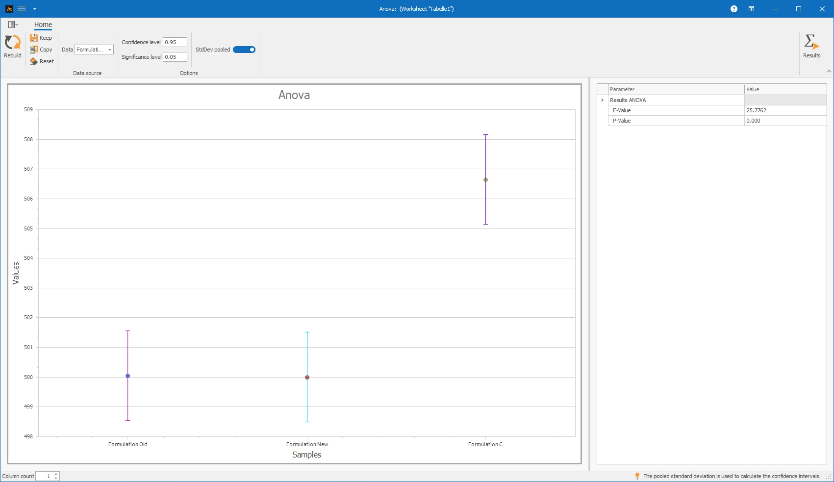
Interpretation of the results:
The calculated p-value is compared with the significance level of 0.05. If the p-value is less than or equal to 0.05, the null hypothesis is rejected. It is then assumed that not all average viscosities of the formulations are equal.
If the p-value is above 0.05, there is no statistical evidence that the mean viscosity differs between the formulations. Since the p-value in our example is 0.000, the null hypothesis is rejected and the alternative hypothesis is accepted.
Explanations of the graphic:
- The points mark the mean viscosities for the individual formulations.
- The error bars represent the 95% confidence interval of the respective mean.
- Overlaps of the confidence intervals provide an initial visual indication. The final decision is made based on the p-value and, if necessary, pairwise comparisons.
Preparation
- Select a continuous measurement (e.g., viscosity).
- Define two or more groups whose means are to be compared (e.g., formulation A, B, and C).
- Set the significance level (usually α = 0.05).
- Check if the data show no strong deviations from the normal distribution.
- Check if the variances of the groups are similarly large.
- Ensure that the measurements were taken independently of each other.
 Use in AlphadiTab
- Select the ANOVA tool in the Analyze phase.
- Select all groups to be compared in the data.
- Conduct the analysis by “Create New”.
Interpretation
- Check if the p-value is less than or equal to the significance level.
p ≤ α → statistically significant difference between at least two means.
p > α → no statistically significant difference between the means.
If the result is significant: conduct pairwise comparisons to determine which groups differ specifically.
Important: ANOVA first tests all groups together. Which groups differ is assessed through pairwise comparisons.
Response time of the IT helpdesk vs. location
In the IT service desk, tickets are processed at multiple locations. The response times are regularly evaluated to identify differences in service quality.
In the example of IT tickets, data from three locations is available. ANOVA is suitable for this case because multiple groups are compared simultaneously. ANOVA reduces the risk of random hits compared to many individual t-tests. For an overall view of the locations, it is therefore generally preferable.
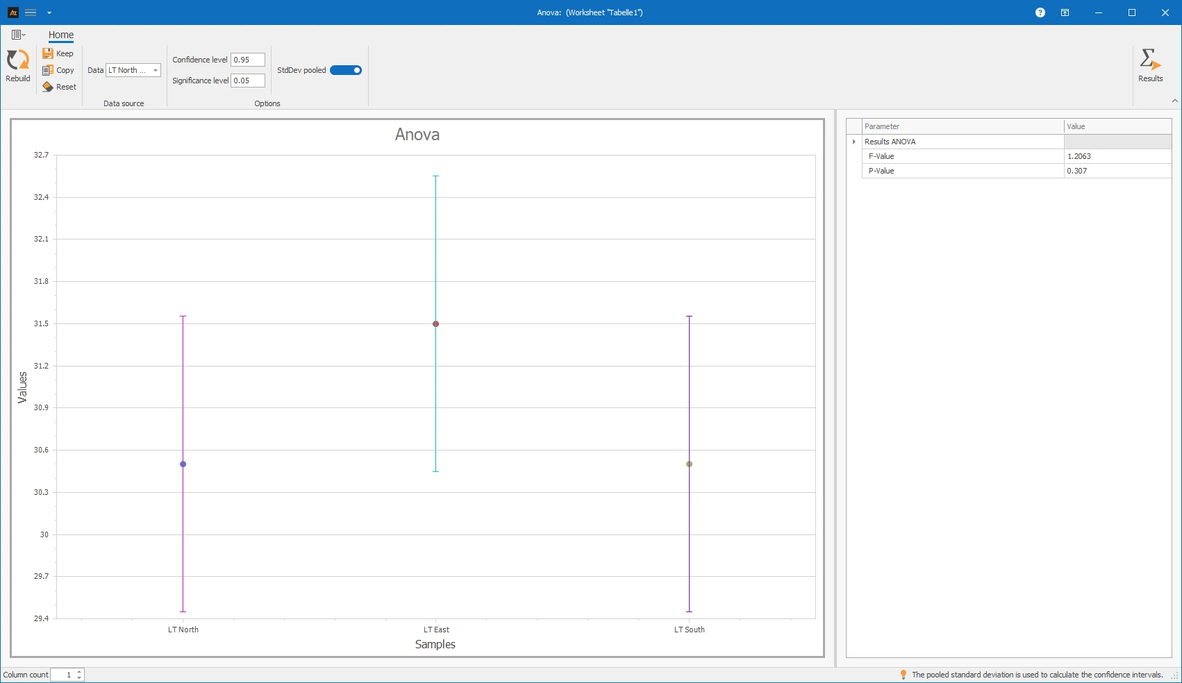
The p-value is above the significance level of 0.05, so the null hypothesis is retained. From a statistical point of view, the average processing times of the locations do not differ significantly.
Lead Time by Region
In sales, customer offers are processed by multiple teams. It should be investigated whether the average lead time (DLT) differs between Team A, Team B, and Team C.
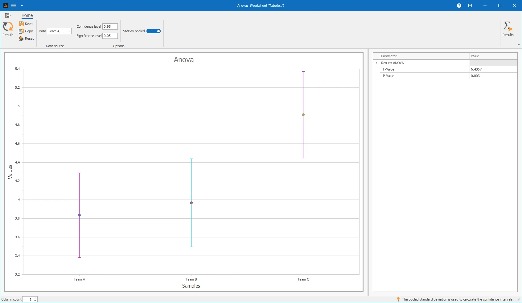
The p-value is below 0.05, so the null hypothesis is rejected. The ANOVA shows a statistically significant difference in the average lead time between the teams. The teams do not process the offers equally fast on average.
Delivery time after logistics center
In the logistics department, customer orders are picked and shipped. Delivery times are compared across multiple logistics centers.
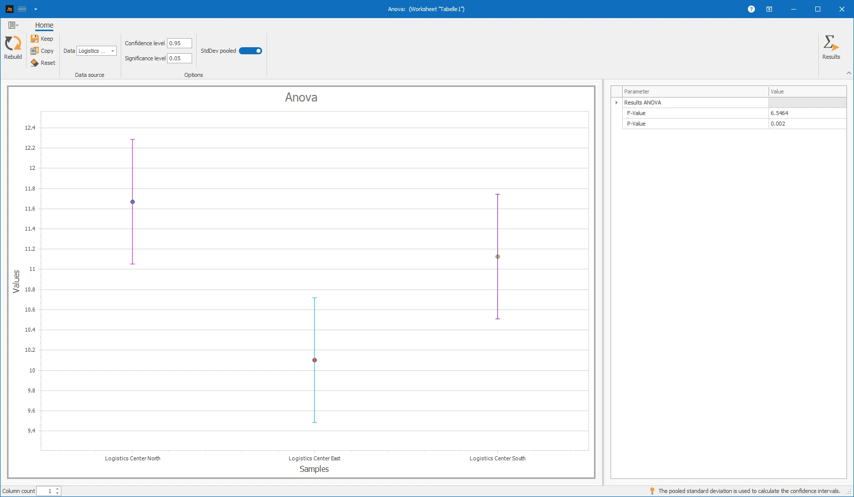
It should be investigated whether the average delivery time (in hours) differs between the logistics centers.
The analysis is carried out using an ANOVA with the logistics center as a factor.
H₀: μ_Center A = μ_Center B = μ_Center C
H₁: At least one mean differs.
Interpretation
The ANOVA shows a statistically significant difference between the average delivery times of the logistics centers (p < 0.05).
Since the p-value is below the significance level of 0.05, the null hypothesis is rejected. At least one logistics center differs in terms of average delivery time.
Supplier comparison
In purchasing, components are sourced from three suppliers. It should be investigated whether the average rejection rate per delivery differs between Supplier A, Supplier B, and Supplier C. The rejection rate is measured per delivery in %.
Note:
ANOVA assumes approximately normally distributed, continuous data. Percentage values like the rejection rate can be discrete, as they arise from count values. With small delivery quantities (e.g., 10 parts per delivery), only a few possible percentage values (0 %, 10 %, 20 % …) arise. In such cases, the assumption of normal distribution may be violated, and ANOVA may not be suitable. With larger delivery quantities with many possible manifestations, ANOVA is generally unproblematic in practice.
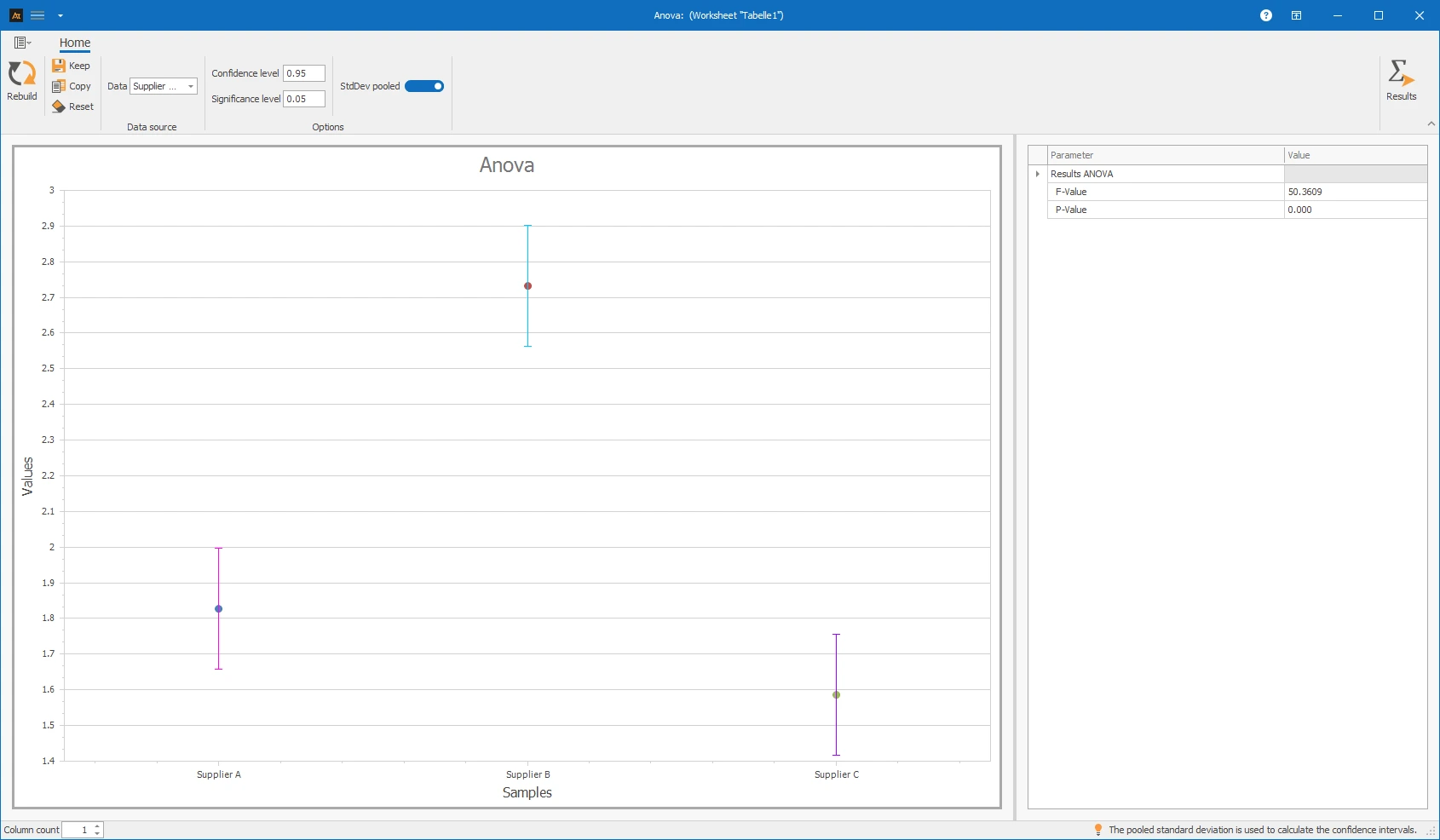
ANOVA shows a statistically significant difference in the average rejection rate between the suppliers (p < 0.05). The null hypothesis is rejected. The suppliers differ in terms of the average rejection rate. Pairwise comparisons then show which suppliers differ specifically.
Forecast deviation
In production planning, demand forecasts are created for different planning periods. To assess the quality of the forecast, the forecast deviation is calculated.
It should be investigated whether the average forecast deviation differs between short-term, medium-term, and long-term planning periods.
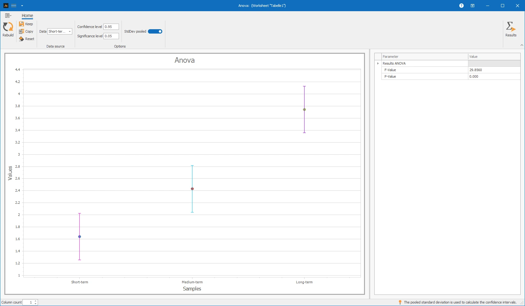
Since the p-value is below the significance level of 0.05, the null hypothesis is rejected. There is thus statistical evidence that the average forecast deviation differs between the planning horizons. The diagram also shows that the deviations increase as the planning horizon becomes larger.
Continuous data: Data collected with a measuring instrument that can have decimal places.
Normally distributed data: Data that can be well described by a normal distribution.
x̄ = Sample mean: Average value of the collected measurement data.
s = Standard deviation: Measure of the dispersion of the data around the mean.
n = Sample size: Number of observations within a sample.
α = Significance level: Preset probability of error (usually 0.05).
p-value: Result of the hypothesis test. Basis for the decision between H₀ and H₁.
F-value: Test statistic of the ANOVA. Ratio of the variance between groups to the variance within groups.
df = Degrees of freedom: Result from the number of groups and observations.
MS = Mean square: Sum of squares divided by the associated degrees of freedom.
Confidence level: Probability that the confidence interval covers the true parameter value (e.g., 95%).
Confidence interval: Range of values that contains the true mean with the chosen confidence level.
Null hypothesis (H₀): All group means are equal.
Alternative hypothesis (H₁): At least one group mean differs from the others.
Factor: Categorical influencing variable by which the measurements are divided into groups.
Levels/Groups: Manifestations of the factor (e.g., formulation A, B, C).
Homogeneity of variance: Assumption that the variances of the groups are similarly large.
H₁: At least one μi differs.
F = MS between groups / MS within groups
The classic one-way ANOVA is calculated using the NMath library. The F-value and p-value are taken from the ANOVA table generated by NMath.