Process Capability Analysis

Purpose of the tool

The process capability analysis aims to evaluate the quality of processes by assessing the position (accuracy) and the spread (precision) of a characteristic using the indicators Cp and Cpk. The higher the Cpk value, the better the process. A process is often considered capable when the Cpk value is 1.33 or higher.

In Lean Six Sigma projects, process capability analysis is typically used in the Measure phase to objectively assess the current performance of a process against the specification limits.

Example: Viscosity Tomato Sauce

You can download the data here: tomato-sauce-viscosity.xlsx File for download

In the production of tomato sauce, viscosity plays a crucial role: If the sauce is too thin or too thick, it does not meet customer expectations. With Cp and Cpk, it can be checked whether the process reliably maintains the desired consistency.

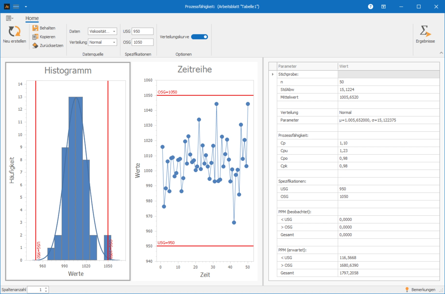
Interpretation of the results:

The evaluation shows a Cp value of 1.10 and a Cpk value of 0.98. The Cpk value is less than the frequently required reference value of 1.33 – the process is therefore not capable.

The Cp value of 1.10 indicates that the process variation is still too large. Since Cpk is also slightly smaller than Cp, there is also a slight positional deviation. However, the main cause is clearly the too high variation.

Explanations of the graphic:

The bars represent the frequency distribution of the measured values.
The line is the normal distribution based on the mean and standard deviation of the actual data.
The narrower the curve, the better the process fits within the specification limits (USL and LSL).

Procedure

Preparation

Select a continuous measurement and collect data (e.g., viscosity).
Check data for normal distribution.
Determine or inquire about specification limits (e.g., LSL = 950, USL = 1050).

Use in AlphadiTab

Select the Measure Phase tool Cp, Cpk.
Select data “Viscosity”.
Specify the specification limits: LSL = 950, USL = 1050.
Select the appropriate distribution.
Conduct analysis by clicking “Create New”.

Interpretation

Check if the process is capable (capable at Cpk ≥ 1.33 or the required minimum value).
Determine if the location, the spread, or both need improvement.

Requirements

Continuous Measurement Data

The measurements must be continuous, meaning they are captured with a measuring instrument and can have decimal places.

Why is this important?

Cp and Cpk assume metric, continuous measurement data. For countable or categorical data, the metrics are not defined.

Normally Distributed Data

The measurements should be well described by a normal distribution (e.g., tested for normal distribution).

Why is this important?

The calculation of Cp and Cpk is based on distribution assumptions. With significant deviations, the metrics become inaccurate.

Choose Appropriate Distribution

For the calculation, it is assumed that the data follow a distribution. Different formulas are stored for different distributions, so the appropriate distribution must be selected (e.g., with the distribution test).

Why is this important?

Without the appropriate distribution, Cp and Cpk no longer match the actual process performance; scrap and risk assessments become inaccurate or misleading.

Suitable Measuring Instrument

The data must be collected with a reliable and suitable measuring instrument for the characteristic.

Why is this important?

If the measuring instrument is not capable, incorrect conclusions about process performance can be drawn – the process may appear incapable, although the deviations are only caused by the measuring instrument.

When are other tools more suitable?

When the data is nominal, ordinal, or discrete (countable)

Other methods (e.g., proportion evaluation)

When the data deviates significantly from the normal distribution or contains significant outliers

Distribution test / suitable distribution

When it needs to be checked in advance whether the data is normally distributed at all

Normal distribution test

When not the capability, but the stability of the process over time is of interest

Control chart (SPC)

Example in Production

Filling Quantity Tomato Sauce

In this example, the filling quantity of the tomato sauce was examined. The filling quantity is recorded with a suitable measuring device to check whether the machine reliably maintains the target quantity of 500 ml.

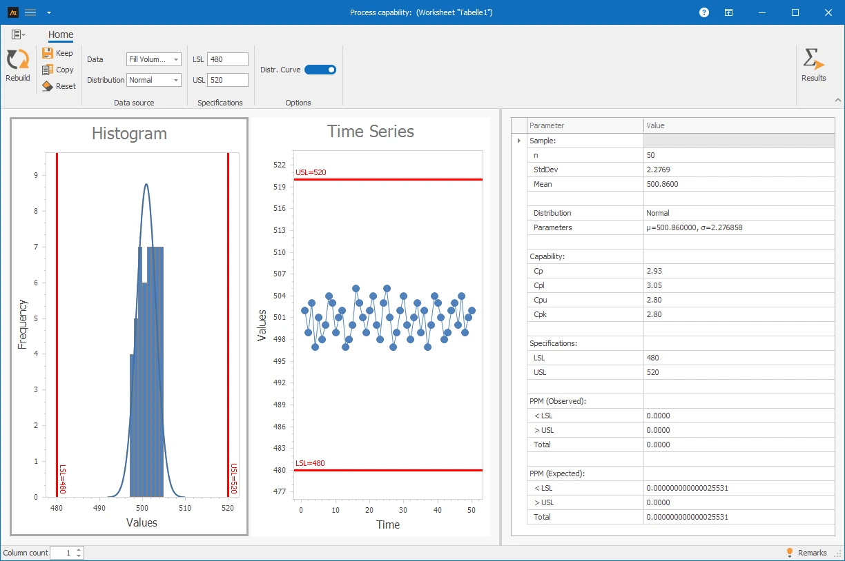
You can download the data here: tomato-sauce-filling-quantity.xlsxFile for download

Determined Key Figures

Cp = 2.93
Cpk = 2.80

Interpretation

The process is capable. Both values are above the frequently required reference value of 1.33. The variation is small enough (Cp high) and the position is good (Cpk ≈ Cp).

→ The process reliably maintains the target quantity – no action required.

Example in Goods Receipt / Logistics

Lead time of an order

In goods receipt, each order goes through a verification step where delivery notes are checked and items are recorded in the system. Missing barcodes, incomplete delivery notes, or inquiries lead to very different processing times.

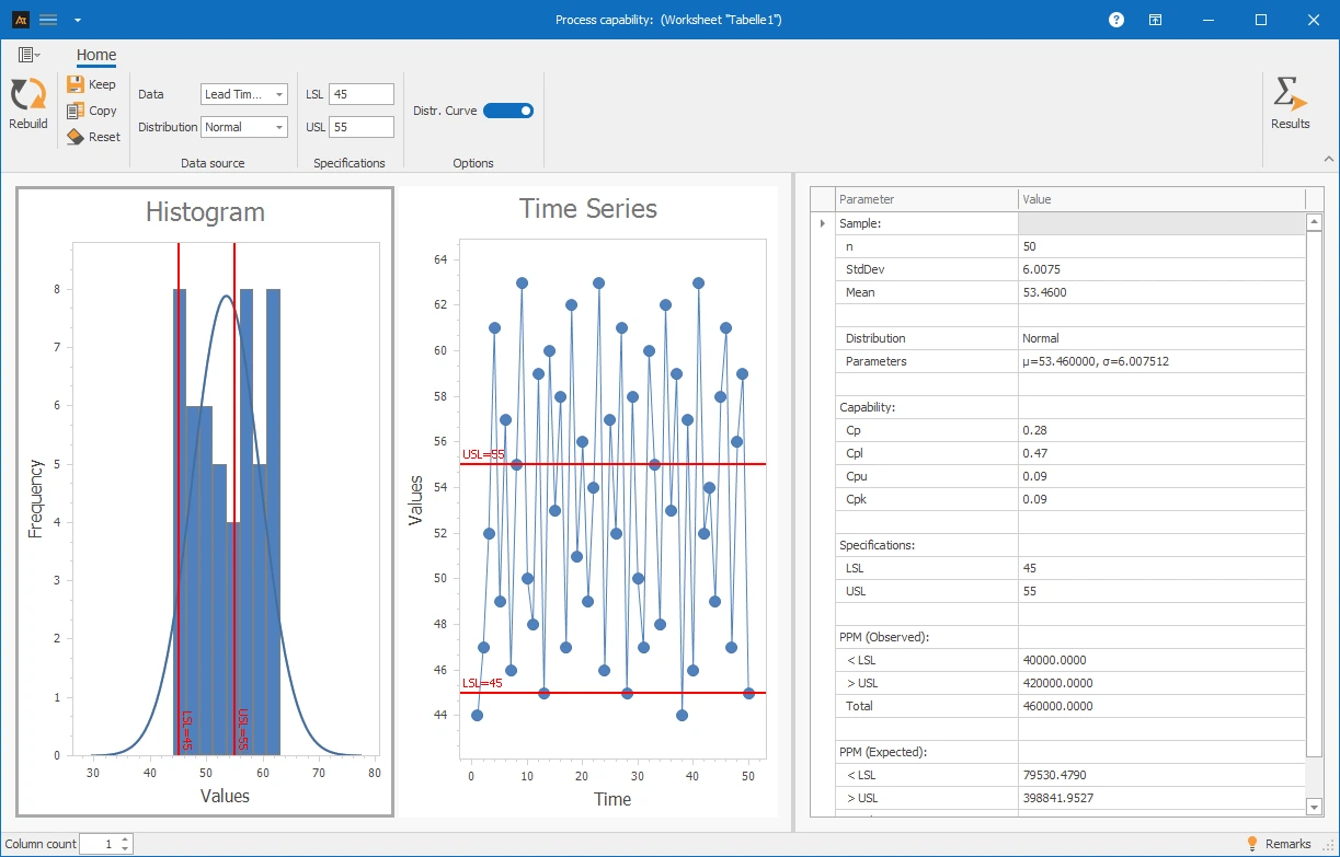
You can download the data here: goods-receipt-throughput-time.xlsxFile for download

Determined Key Figures

Cp = 0.28
Cpk = 0.09

Interpretation

The process is not capable. Cp < 1.33 → Variation too large, lead times fluctuate greatly. Cpk < Cp → additionally a location problem.

→ Reduce variation and stabilize process location to get lead times under control.

Example in IT support

Response time requests

Many different requests are received daily at the IT service desk. While simple cases are processed quickly, the response is delayed for more complex tickets – although the response time should not exceed 35 minutes.

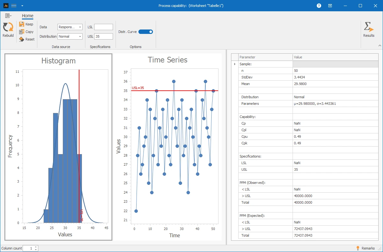
You can download the data here: it-service-response-time.xlsxFile for download

Determined key figures

Cp: not calculable, as only one specification limit is available
Cpk = 0.49

Interpretation

The process is not capable, as the Cpk value is significantly below the required minimum value of 1.33. Since only an upper specification limit is defined, optimization can be achieved through both lower variability and better positioning.

→ Standardize the processing process to reliably bring response times below the limit.

Terms

Continuous data: Data collected with a measuring instrument that can have both units and decimal places.

Normally distributed data: Data that can be well described by a normal distribution (e.g., tested for normal distribution).

OSG / OTG: Upper specification or tolerance limit – the maximum allowable value for the target variable.

USG / UTG: Lower specification or tolerance limit – the minimum allowable value for the target variable.

Cp: Capability index that evaluates the spread of the process in relation to the specification limits.

Cpk: Capability index that evaluates both the spread and the position of the process in relation to the specification limits.

x̄ = Sample mean: Average value of the collected measurement data.

s = Standard deviation: Measure of the spread of the data around the mean.

Formulas

Mean

x̄ = (1/n)·∑_i=1ⁿ x_i

Standard Deviation

s = √((1/(n−1))·∑_i=1ⁿ (x_i − x̄)²)

Capability Index Cp

C_p = (USL − LSL) / (6·s)

Capability Index Cpk

C_pk = min((USL − x̄)/(3·s), (x̄ − LSL)/(3·s))

Notation

x̄ = Sample mean

s = Sample standard deviation

n = Sample size

x_i = i-th measurement