


The t-test is used to determine whether the means of two groups differ statistically significantly.
It is used to assess whether an observed difference between two groups goes beyond random fluctuations.
The decision is made by comparing the p-value with the predetermined significance level (usually α = 0.05):
- p ≤ α → accept H₁ (reject H₀)
- p > α → retain H₀

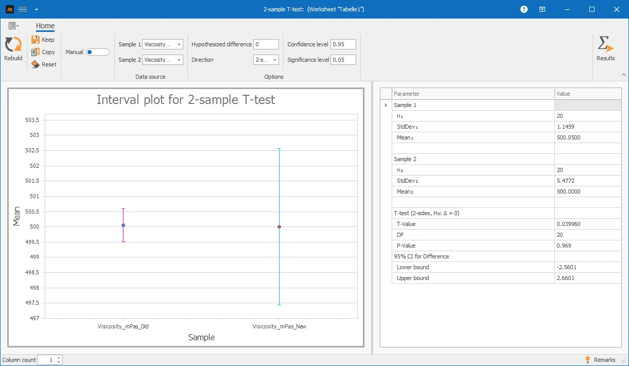
In product development, a new recipe for tomato sauce is being tested. The goal is to check whether the viscosity of the new recipe differs on average from the previous recipe. For this purpose, viscosity measurements are carried out on samples of the old and new recipe.
Interpretation of the results:
The determined p-value is significantly above the significance level of 0.05, so the null hypothesis is retained. There is no evidence that the average viscosity of the new recipe differs from the previous one.
Explanations of the graphic:
- The points mark the mean values of viscosity for the old and new recipe.
- The error bars represent the 95% confidence interval of the mean.
- The significant overlap of the confidence intervals shows that there is no statistically significant difference.
Preparation
- Select a continuous measurement (e.g., viscosity).
- Define two groups whose means are to be compared.
- Set the significance level (usually α = 0.05).
- Check if the data shows no strong deviations from the normal distribution.
- Ensure that the measurements were collected independently.
 Use in AlphadiTab
- Select the 2-sample t tool in the Analyze phase.
- Select the first group for sample 1.
- Select the second group for sample 2.
- Conduct the analysis by Create New.
Interpretation
- Check if the p-value is less than or equal to the significance level.
- p ≤ α → statistically significant difference in means.
- p > α → no statistically significant difference in means.
- The interpretation refers exclusively to the mean.
The t-test offers two main settings: the type of data input and the direction of the hypothesis.
Manual input: The comparison is based on manually entered standard deviations and sample sizes of two samples.

Non-manual input (dataset): The comparison is based on the selected data columns.

H₀: μ₁ − μ₂ = Δ₀ | H₁: μ₁ − μ₂ ≠ Δ₀
Select two-sided if you want to test whether the means of the two samples differ without specifying a particular direction. Useful when there is no specific expectation about the direction of the difference. Example: Do the average test scores of Group A and Group B differ?
H₀: μ₁ − μ₂ = Δ₀ | H₁: μ₁ − μ₂ > Δ₀
Select greater if you want to test whether the mean of the first sample is greater than that of the second. It only tests if sample 1 has significantly higher values. Example: Is the average revenue after an advertising campaign higher than before?
H₀: μ₁ − μ₂ = Δ₀ | H₁: μ₁ − μ₂ < Δ₀
Select smaller if you want to test whether the mean of the first sample is smaller than that of the second. It only tests if sample 1 has significantly lower values. Example: Is the average processing time after an optimization lower than before?
Filling Quantity Tomato Sauce
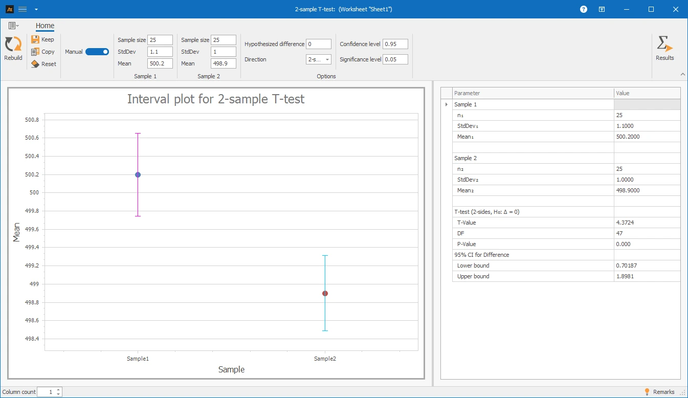
In production, two filling machines are used. It should be investigated whether the average filling quantity differs between Machine A and Machine B. The measurement data for both machines are available in summarized form:
- Machine A: n = 25, Mean = 500.2 ml, Standard Deviation = 1.1 ml
- Machine B: n = 25, Mean = 498.9 ml, Standard Deviation = 1.0 ml
The comparison of the means is done using a t-test (2 samples).
Interpretation
The t-test shows a statistically significant difference in the average filling quantity between the two machines. The p-value is below 0.05, so the null hypothesis is rejected.
→ The machines differ in the mean filling quantity.
Response time requests
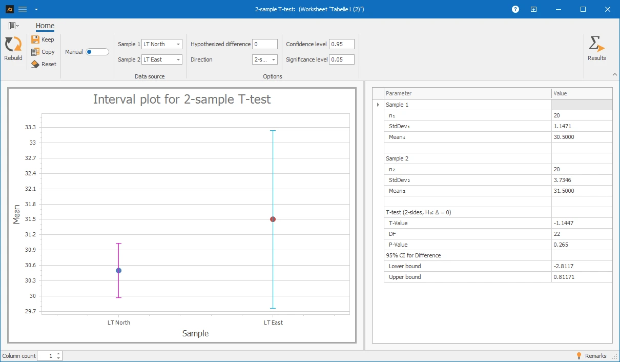
In the IT service desk, tickets are processed at multiple locations. Response times are regularly evaluated to identify differences in service quality. In the example, data from three locations is available. The t-test (2 samples) is basically only suitable for comparing two groups. For more than two locations, there are two approaches:
Pairwise comparisons with the t-test: Each location can be compared pairwise with the others (e.g., A vs. B, A vs. C, B vs. C).
Alternative – Analysis of variance (ANOVA): If all locations are to be considered simultaneously, an ANOVA is the more suitable tool. It checks whether there is at least one significant difference between the means without having to perform multiple individual tests.
Note: With multiple pairwise t-tests, the risk of random hits increases.
Interpretation
The t-test shows no statistically significant difference between the average processing times of the locations DLZ North and DLZ East. The p-value is above 0.05, so the null hypothesis is retained.
→ No mean difference; prefer ANOVA for more than two locations.
Sales Rate by Region
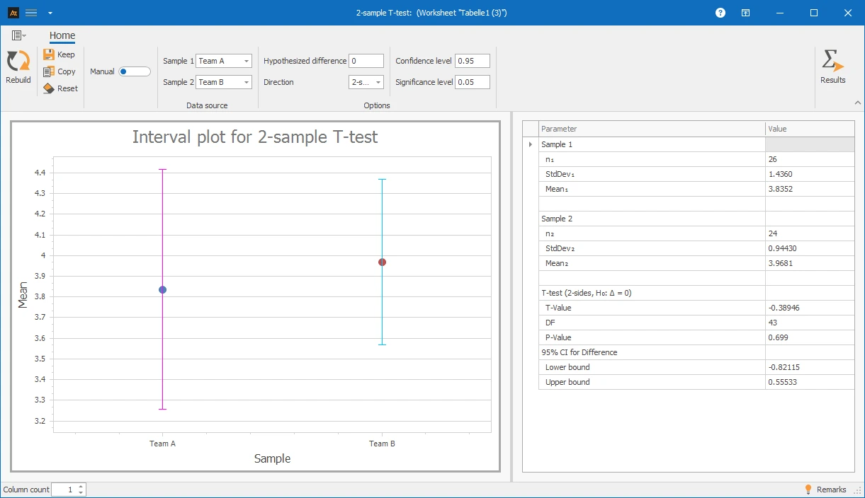
In sales, customer offers are processed by two teams. It should be investigated whether the average lead time (DLT) differs between Team A and Team B.
Interpretation
The t-test shows no statistically significant difference in the average lead time between the two teams. The p-value is above 0.05, so the null hypothesis is retained.
→ Both teams process the offers equally fast on average.
Delivery time after logistics center
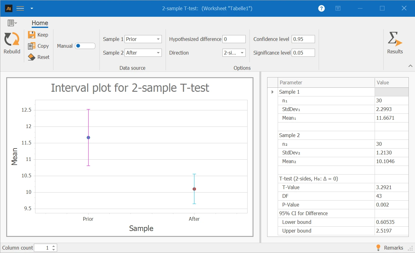
In the logistics department, customer orders are picked and shipped. To increase efficiency, new forklifts have been introduced. It should be investigated whether the average delivery time (in hours) has decreased after the introduction. The analysis is carried out as a one-sided t-test (direction “greater”).
H₀: μBefore − μAfter = 0 | H₁: μBefore − μAfter > 0
Interpretation
The one-sided t-test shows a statistically significant difference (t = 3.29; p = 0.001). The average delivery time before the introduction is significantly higher than afterwards.
→ The new forklifts have significantly reduced the average delivery time.
Supplier Comparison
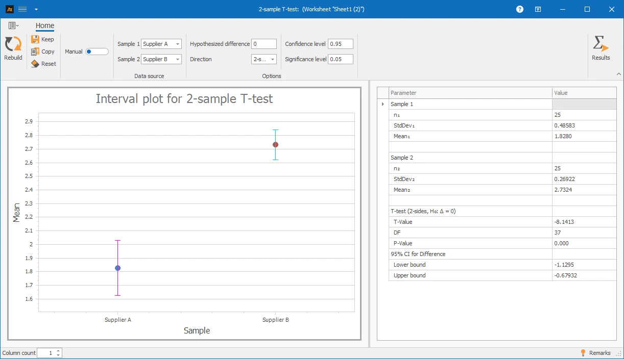
In purchasing, components are sourced from two suppliers. It should be investigated whether the average rejection rate per delivery differs between Supplier A and Supplier B (measured in %).
Note: The t-test assumes approximately normally distributed, continuous data. Percentage values can be discrete; with small delivery quantities, the normal distribution assumption may be violated. With larger delivery quantities, the t-test is generally unproblematic in practice.
Interpretation
The t-test shows a statistically significant difference in the average rejection rate between the suppliers (p < 0.05). The null hypothesis is rejected.
→ Supplier A has the better (lower) rejection rate.
Forecast deviation
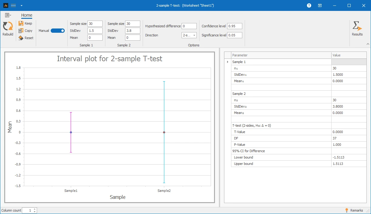
In production planning, demand forecasts are created for different planning periods. To assess the quality of the forecast, the forecast deviation is calculated. It is examined whether the average forecast deviation differs between short- and long-term planning periods:
- Short-term horizon: n = 30, mean = 0.0 %, standard deviation = 1.5 %
- Long-term horizon: n = 30, mean = 0.0 %, standard deviation = 3.8 %
Interpretation
The t-test for two independent samples shows that the mean forecast deviations do not differ statistically significantly. Since the p-value is above 0.05, the null hypothesis is not rejected.
→ No difference in the mean forecast deviation between short- and long-term.
t-value: Test statistic of the t-test. Ratio of the observed mean difference to the data's variability.
p-value: Result of the hypothesis test. Basis for the decision between H₀ and H₁.
α = Significance level: Preset probability of error (usually 0.05).
H₀ (Null hypothesis): The means of the two groups are equal.
H₁ (Alternative hypothesis): The means of the two groups differ.
df = Degrees of freedom: Derived from the sample sizes of both groups.
Confidence interval: Range of values that contains the true mean difference with the chosen confidence level.
Two-tailed / one-tailed: Indicates whether a difference is tested in both or only one direction.