


The test of proportions (2 samples) is used to check whether the proportions of two groups differ statistically significantly.
It is used to assess whether an observed difference between two proportions goes beyond random fluctuations. The basis is a hypothesis test for binary events (event / no event).
- p ≤ α → accept H₁ (reject H₀)
- p > α → retain H₀
A manufacturer of tomato sauce wants to check if the proportion of leaky jars differs between two filling lines.
- Line A: 30 out of 100 jars are leaky
- Line B: 50 out of 100 jars are leaky
Using the test of proportions (2 samples), it is checked whether the observed difference is statistically significant.
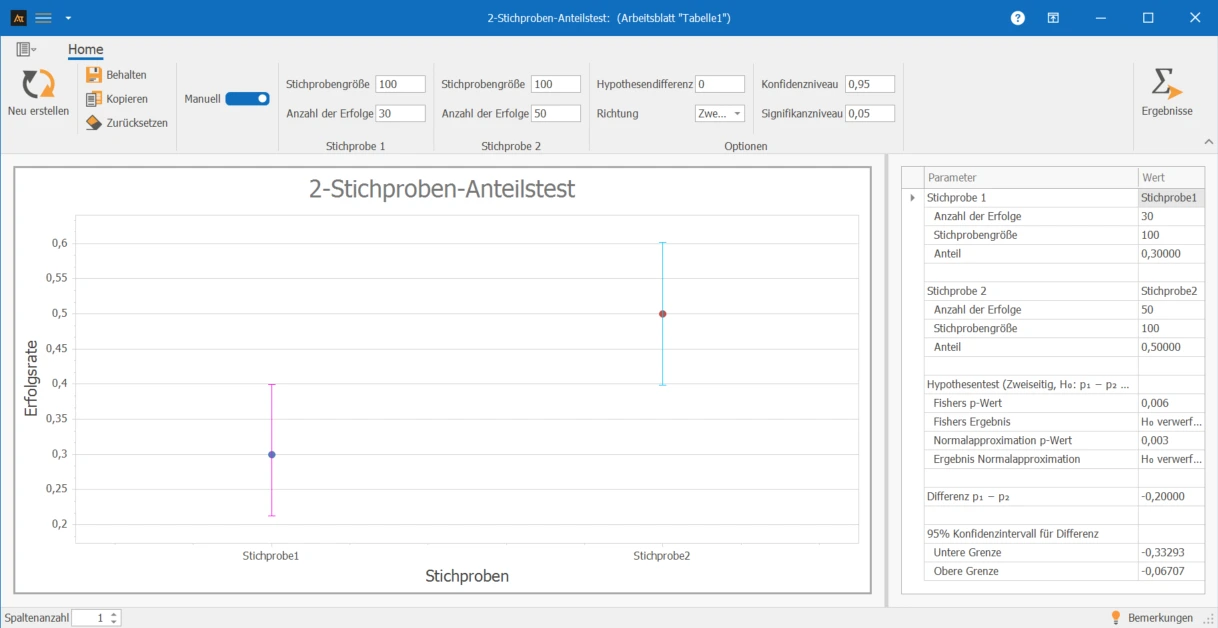
Interpretation of the results:
The calculated p-value is below the significance level of 0.05, so the null hypothesis is rejected. There is statistical evidence that the probability of leaky jars is not the same on the two lines.
Explanations of the graphic:
- The points mark the observed sample proportions of the two filling lines.
- The error bars represent the 95% confidence interval of the respective proportions.
- If the confidence intervals overlap little to not at all, this indicates a statistically significant difference.
Preparation
- Select a binary event (e.g., Lid tight: Yes/No).
- Define two groups whose proportions are to be compared.
- Set the significance level α (usually α = 0.05).
- Ensure that observations within and between groups were collected independently.
 Usage in AlphadiTab
- Select the tool Test of Proportions, 2 Samples in the Analyze phase.
- Activate the slider on Manual (or select data columns).
- Specify the number of events and the number of trials under Sample 1.
- Specify the number of events and the number of trials under Sample 2.
- Conduct the analysis by Create New.
Interpretation
- Check if the p-value is less than or equal to the significance level.
- p ≤ α → statistically significant difference in proportions.
- p > α → no statistically significant difference in proportions.
- The interpretation refers to proportions – not means.
- The p-value of Fisher's exact test is valid for all sample sizes.
The test of proportions offers two main settings: the type of data input and the direction of the hypothesis.
Manual input: The comparison is based on the number of events and the number of trials in both samples.


H₀: p₁ − p₂ = Δ₀ | H₁: p₁ − p₂ ≠ Δ₀
Select two-sided if you want to check whether the proportions of the two samples differ without specifying a particular direction. Example: Does the rate of leaking jars differ between filling line A and B?
H₀: p₁ − p₂ = Δ₀ | H₁: p₁ − p₂ > Δ₀
Select greater if you want to check whether the proportion of the first sample is greater than that of the second. Example: Is the proportion of timely delivered pallets at the North site higher than at the South site?
H₀: p₁ − p₂ = Δ₀ | H₁: p₁ − p₂ < Δ₀
Select smaller if you want to check whether the proportion of the first sample is smaller than that of the second. Example: Is the proportion of incorrectly labeled jars in shift A lower than in shift B?
Rejection rate – Filling line A vs. Filling line B
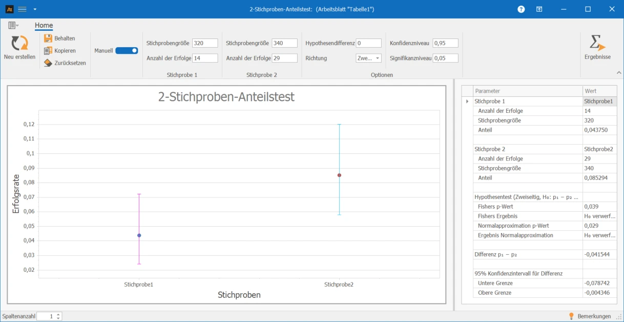
In the production of tomato sauce, two filling lines are used. It is being investigated whether the proportion of leaky jars differs between machine A and machine B. The data is available in summarized form:
- Machine A: 14 leaky jars out of 320 tested
- Machine B: 29 leaky jars out of 340 tested
Interpretation
The proportion test shows a statistically significant difference in the rejection rate (p < 0.05). Since neither events nor counter-events are less than 5, the normal approximation is permissible; it leads to the same result here as the exact Fisher test.
→ Significant difference in the rejection rate between the machines.
Success rate of new lid geometry
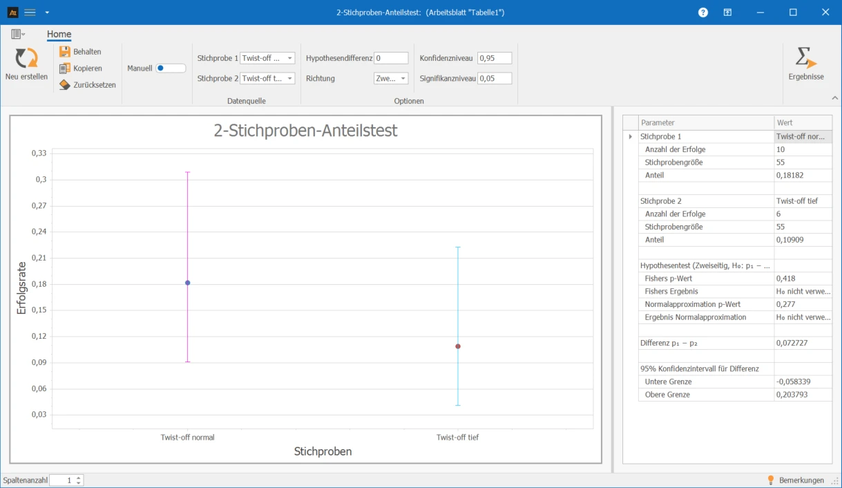
A new lid geometry is being tested in development. It is being investigated whether the proportion of passed leak tests differs between the previous and the new variant.

Interpretation
The test shows no statistically significant difference in the success rate of the leak test (p > 0.05). The null hypothesis is retained.
→ No difference between old and new lid geometry.
First-time resolution rate of service tickets
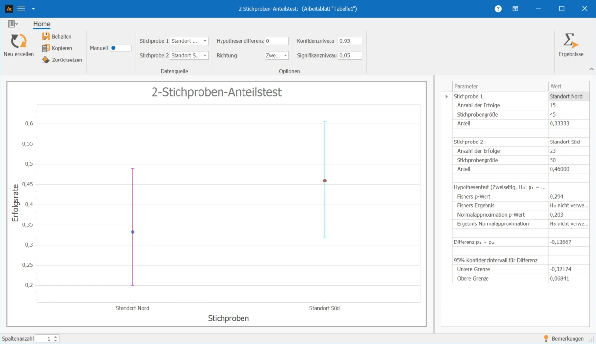
In IT service, it is examined whether the proportion of directly resolved service tickets differs between the North and South locations.
Interpretation
The test shows no statistically significant difference in the first-time resolution rate between the locations (p > 0.05). The null hypothesis is retained.
→ No difference in the first-time resolution rate between North and South.
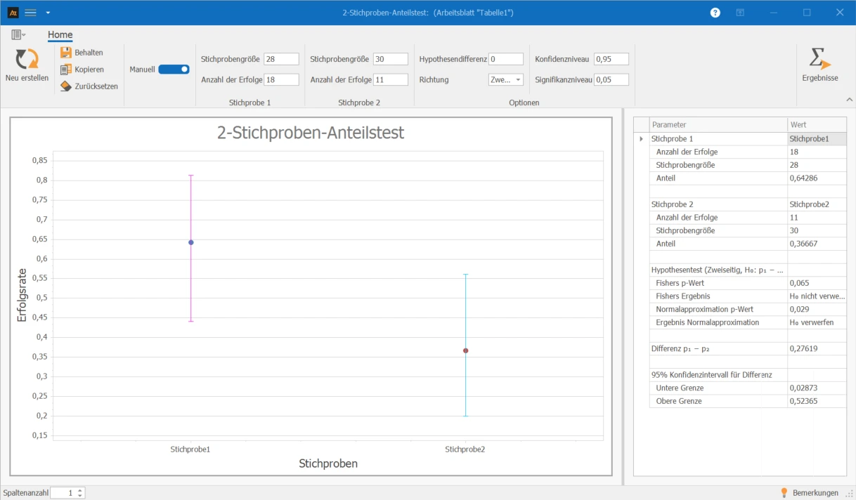
Loss rate by sales approach
In sales, it is examined whether the proportion of lost offers differs between sales approach A and sales approach B.
Interpretation
There are two p-values. The normal approximation indicates a significant difference (p = 0.029), while the exact Fisher test is above the significance level. Since in both samples events and counter-events are at least 5 each, the condition for the normal approximation is met – it is used for assessment, and the null hypothesis is rejected.
→ Normal approximation (p = 0.029) → significant difference in loss rate.
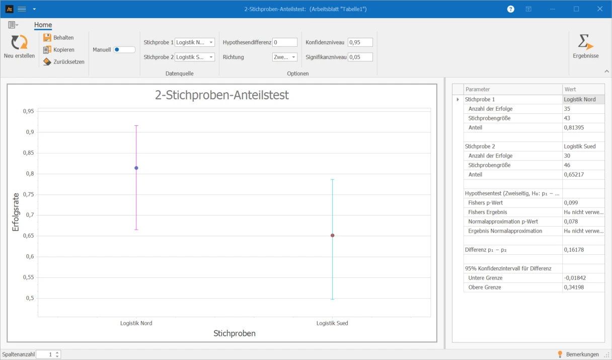
Punctually provided pallets by location
In logistics, deliveries are prepared at two locations. It is checked whether the North location achieves a higher proportion of punctually provided pallets than the South location. The analysis is carried out as a one-sided test (direction "greater").
H₀: pNorth − pSouth = 0 | H₁: pNorth − pSouth > 0
Interpretation
The test shows no statistically significant difference in the proportion of punctually provided pallets between the locations (p > 0.05). The null hypothesis is retained.
→ The North location is not significantly better than the South location.
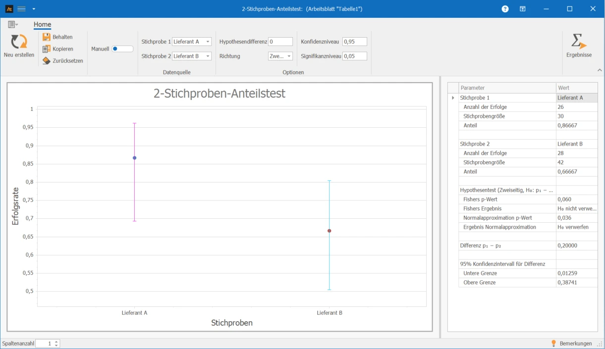
Supplier Comparison for Screw Caps
In purchasing, screw caps are sourced from two suppliers. It is examined whether the proportion of damaged deliveries differs between Supplier A and Supplier B.
Note: For very small numbers of events or non-events, the normal approximation may be inaccurate – in such cases, the exact method (Fisher) is important.
Interpretation
There are two p-values. The normal approximation would suggest rejection, but its assumption is not met here (in sample 1, the counter-events are less than 5). Therefore, the decision is based on the exact Fisher test – this shows no significant difference, the null hypothesis is retained.
→ Normal approximation assumption violated → Fisher is crucial → no significant difference.
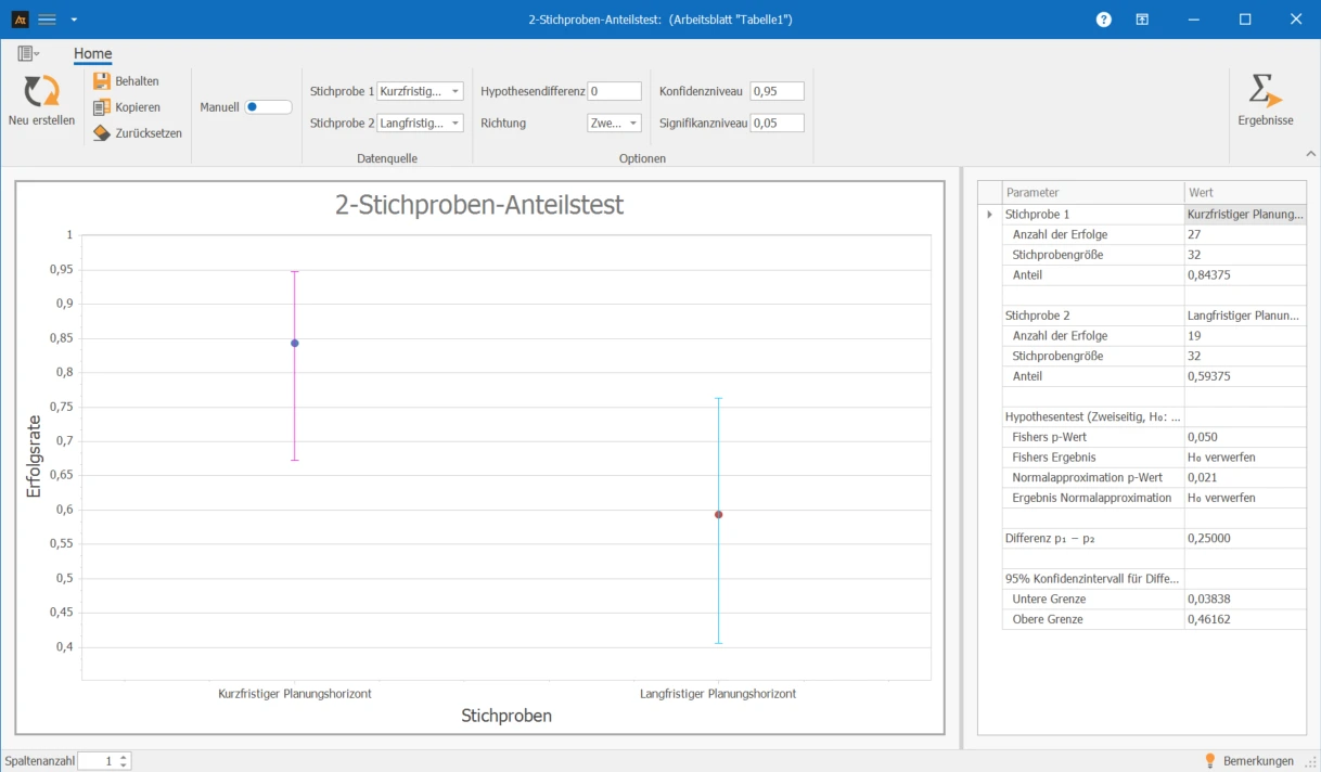
Forecast Hit Rate by Planning Horizon
The planning examines whether the proportion of sufficiently accurate sales forecasts differs between short-term and long-term planning horizons.
Interpretation
Both the exact Fisher test and the normal approximation are at or below the significance level of 5 %. Both tests indicate a significant difference; the null hypothesis is rejected.
→ Significant difference in forecast hit rate between the horizons.
p₁, p₂: Observed sample proportions of the two groups.
α = Significance level: Preset error probability (usually 0.05).
H₀ (Null hypothesis): The proportions of the two groups are equal.
H₁ (Alternative hypothesis): The proportions of the two groups differ.
p-value: Result of the hypothesis test.
Fisher's exact test: Exact method, valid for all sample sizes, even with small event numbers.
Normal approximation: Approximation method, suitable when event and counter-event numbers are each ≥ 5.
Confidence interval: Range of values that contains the true proportion with the chosen confidence level.