


The distribution test tool is used to compare a selected data series with several theoretical distributions. It helps to identify which distribution best describes the measurements and whether the data is suitable for further statistical analyses with a specific distribution assumption.
The result is not a definitive "proof" for a distribution. A high p-value merely means that the Anderson-Darling test does not find a statistically significant deviation from the chosen distribution. The technical plausibility, process reference, and probability network must always be considered.

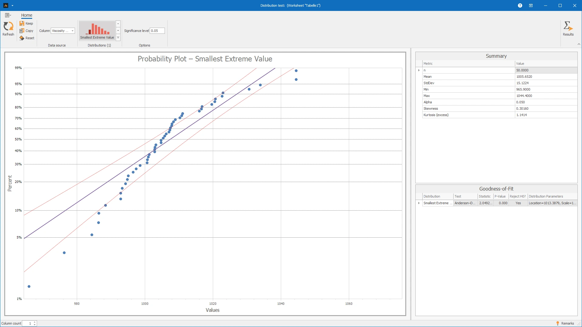
During the production of tomato sauce, viscosity values are regularly recorded. Viscosity describes how thick the sauce is. It is important so that the product can be filled evenly and always has the same consistency for the customer.
Before further analyses are conducted, it should be checked which of the selected distributions can meaningfully describe the measured viscosity values. For this purpose, the data are compared with the distribution tests for the distributions Normal, Lognormal, Loglogistic and Logistic.
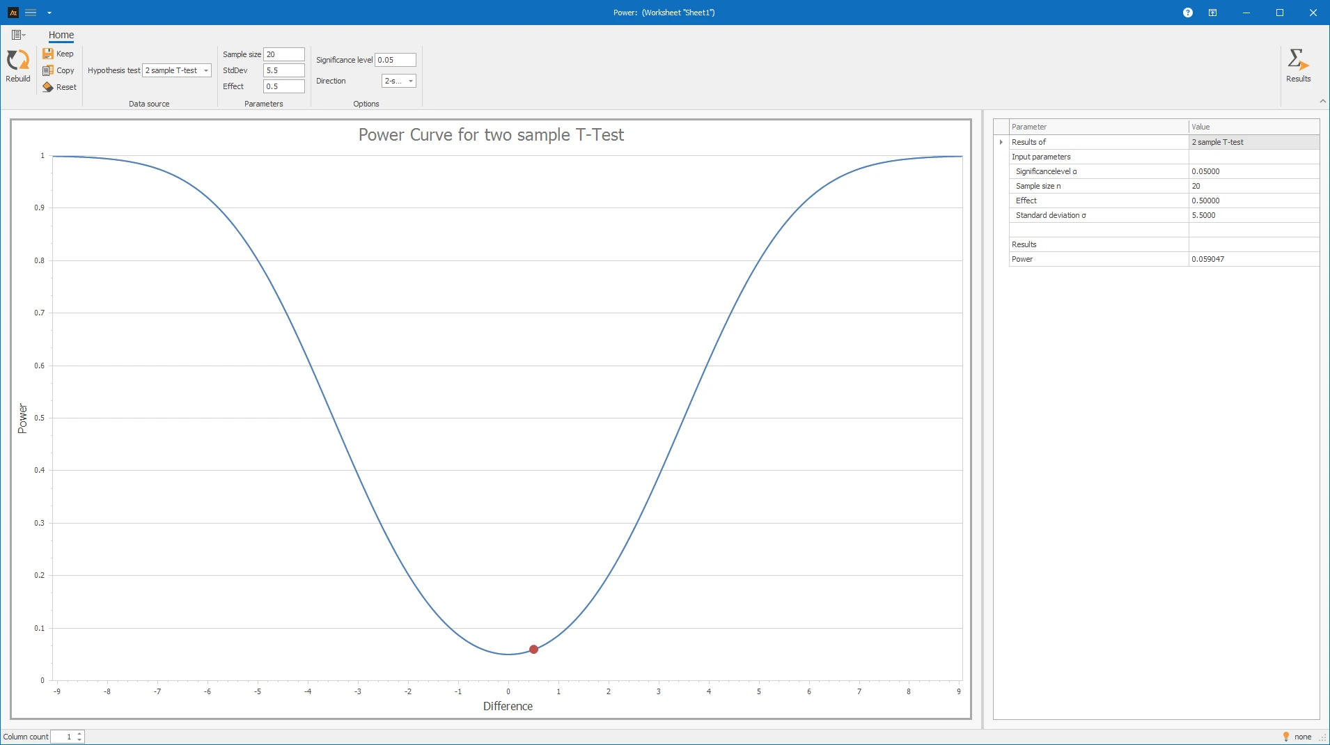
Explanations of the results:
Probability plots
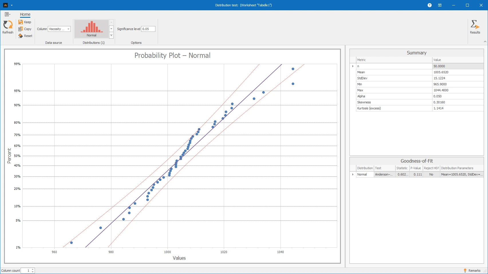
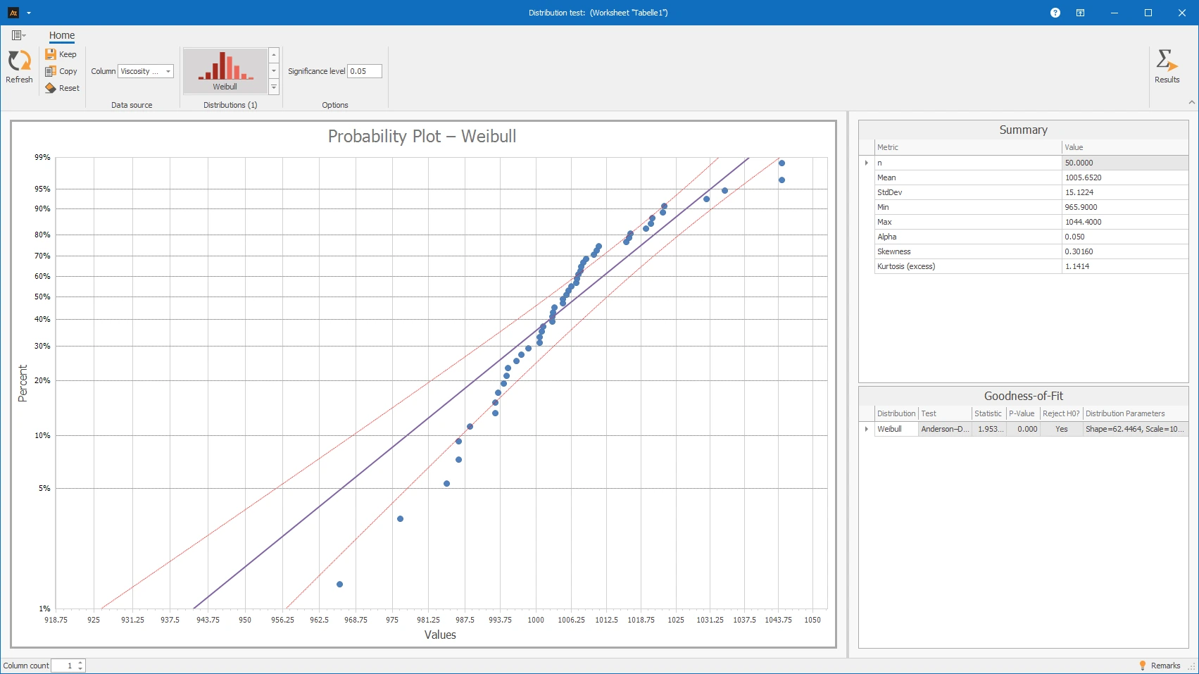
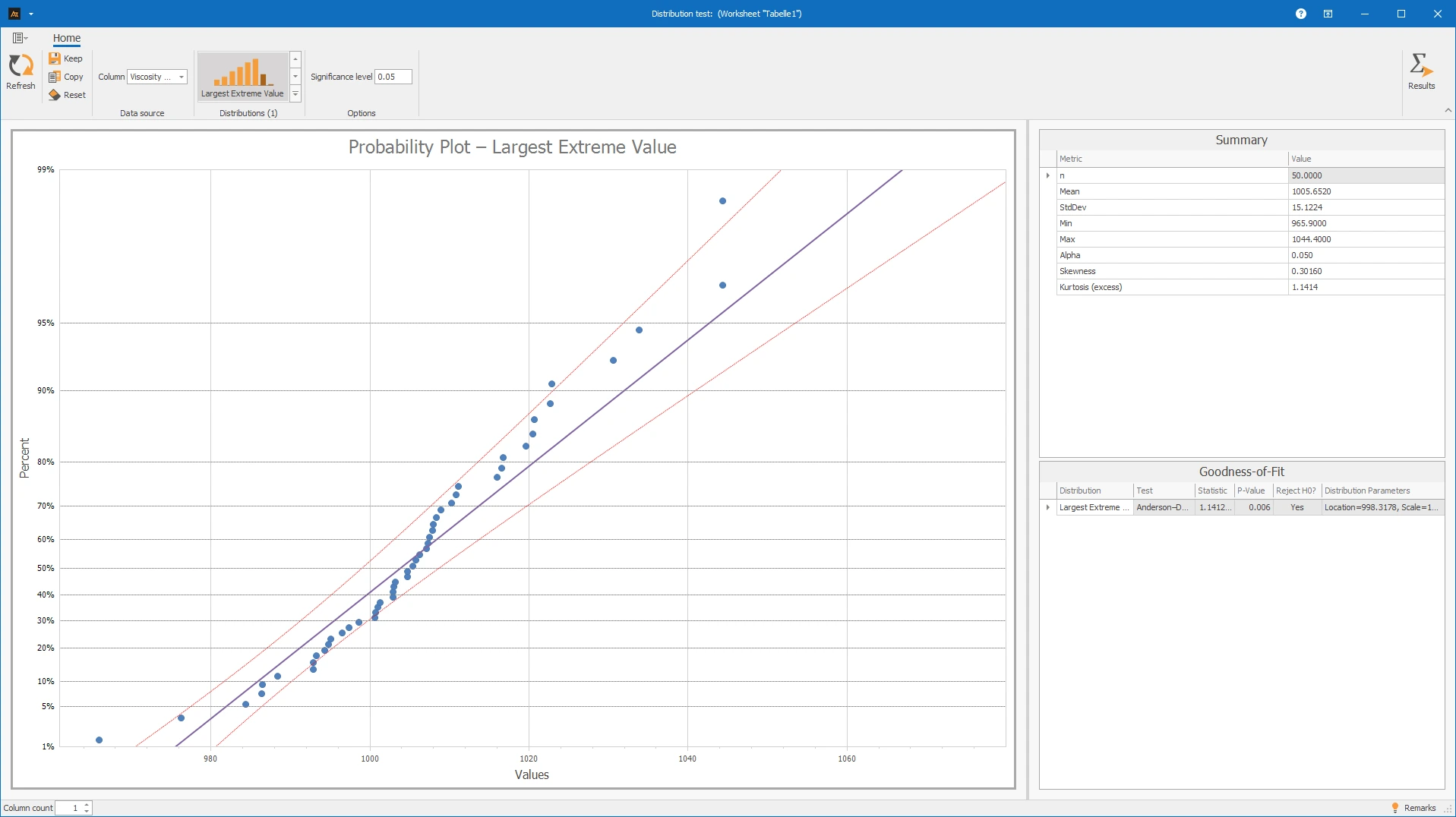
For each successfully calculated distribution, the distribution test generates its own probability plot. In it, the sorted measured values are compared with the values that would be expected under the respective theoretical distribution.
- If the points are close to the drawn line, the chosen distribution fits the data well. The more the points deviate from the line, the worse this distribution describes the data.
- Curved patterns, S-shapes, significant outliers, or deviations in the edge areas indicate that the data do not fit well with the tested distribution.
- When comparing multiple distributions, not only the p-value should be considered. It is also important whether the probability plot shows a plausible, calm pattern and whether the distribution fits the characteristic technically.
The line can be understood as a template: The better the points fit the template of the distribution, the more suitable this distribution is as a model for the data.
Anderson-Darling test
The distribution test uses the Anderson-Darling test as a computational goodness-of-fit test. The test checks whether the measured values fit the selected distribution. It is performed for all supported distributions that can be calculated with the available data.
The test outputs a test statistic and a p-value for each distribution:
- p-value greater than alpha: There is no statistical evidence that the data deviate from this distribution. → The distribution can be considered a possible model.
- p-value less than or equal to alpha: The test finds significant deviations. → The null hypothesis is rejected; the tested distribution does not statistically fit the data sufficiently.
Why is the Anderson-Darling test used? It is particularly sensitive to deviations in the edge areas of the distribution. This is where outliers or extreme values often occur, which are important for quality, process, and lifetime analyses.
Interpretation of the results:
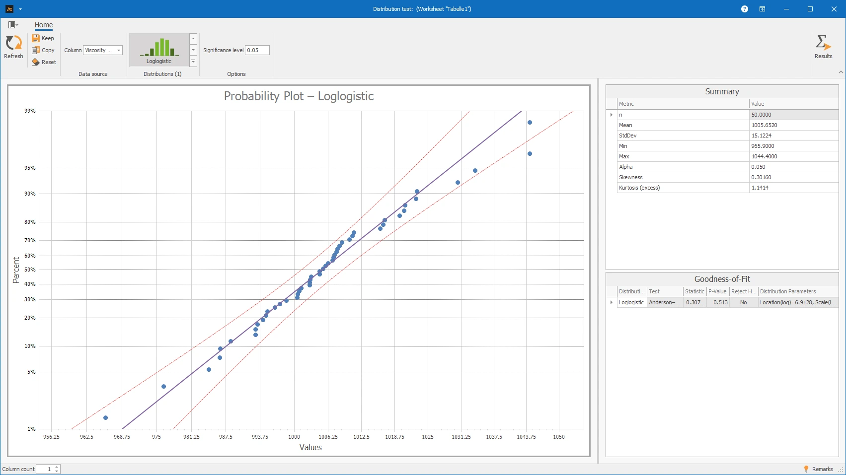
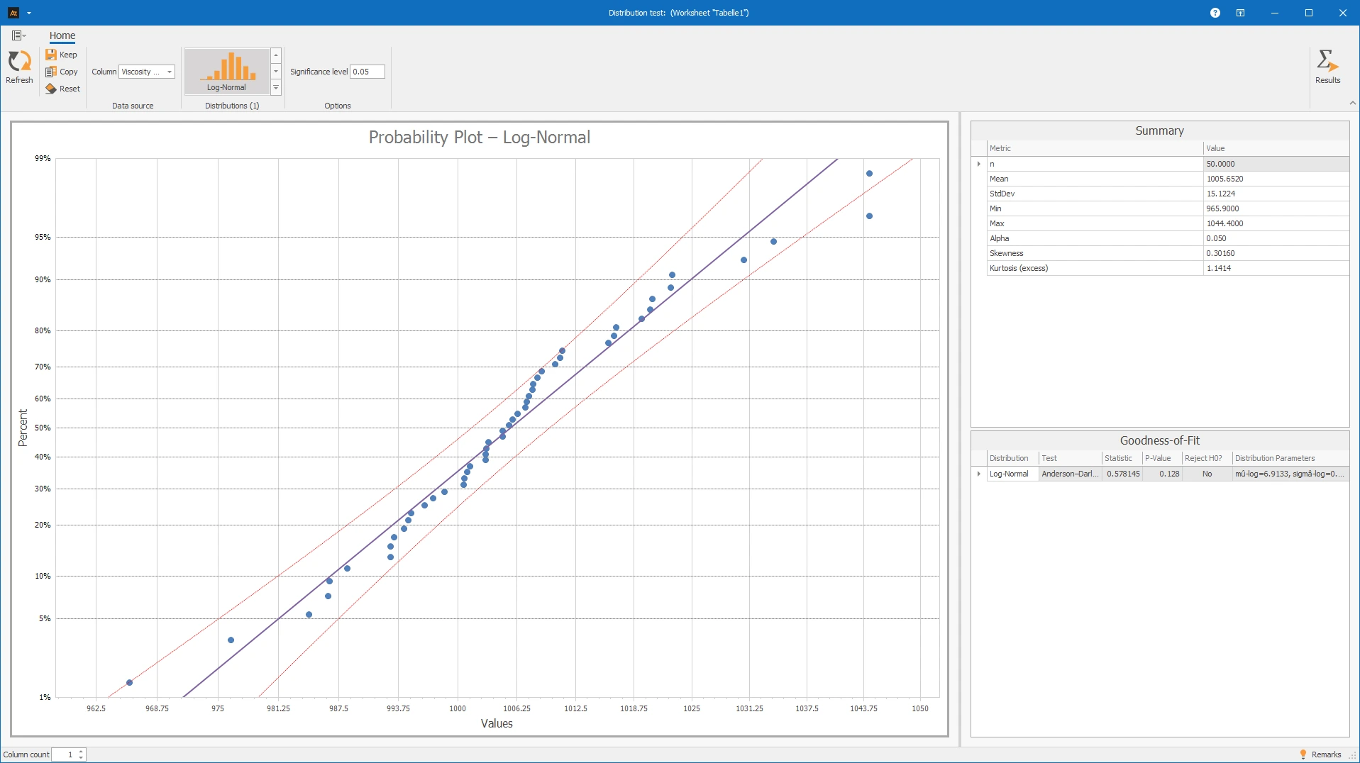
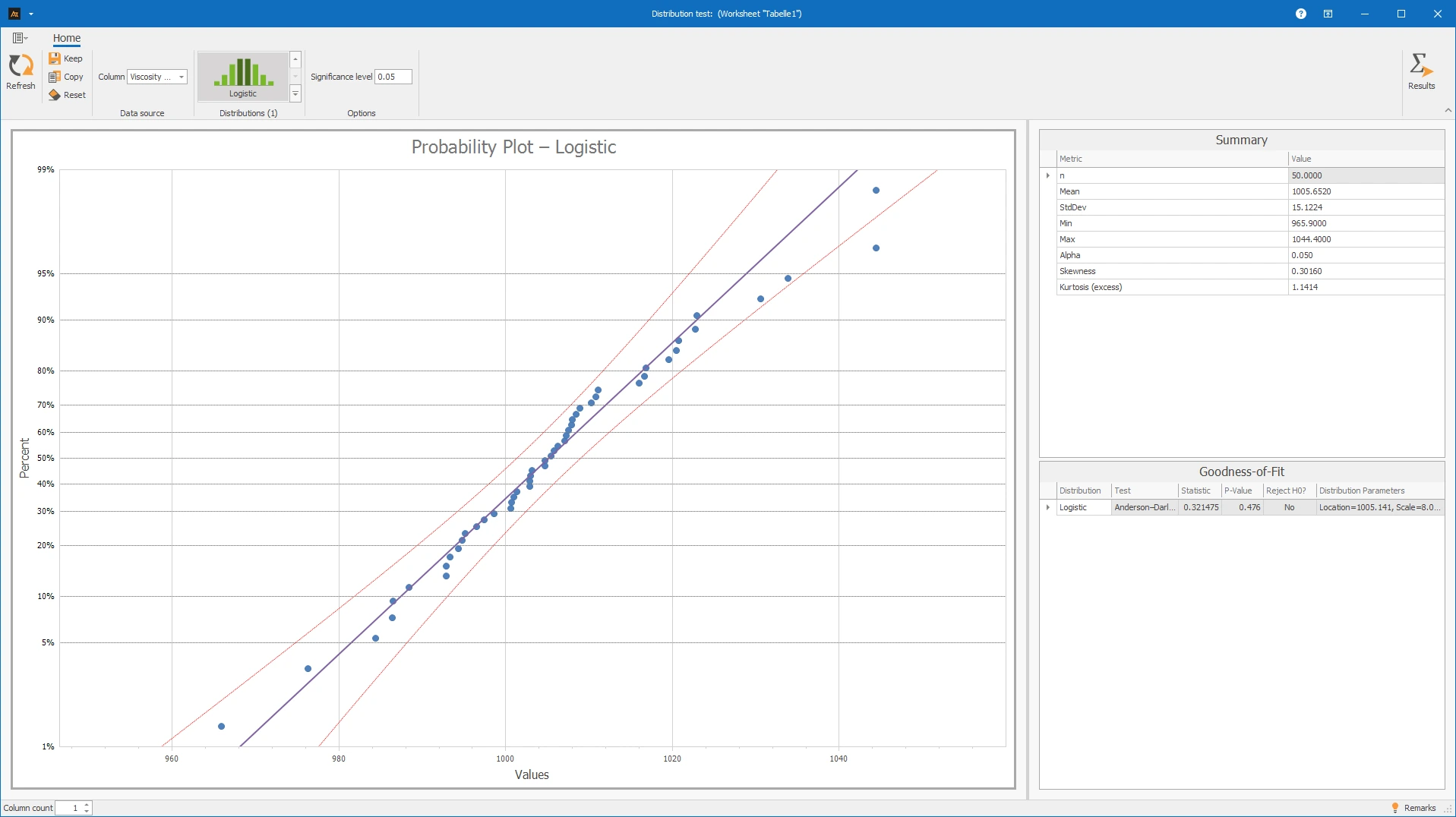
The viscosity values were compared with the distributions Normal, Lognormal, Loglogistic, and Logistic. For all four distributions, the p-value is greater than 0.05. Therefore, the null hypothesis is not rejected for any distribution. There is no statistical evidence that the data significantly deviate from any of the tested distributions.
The probability plots also show that the points mostly lie close to the lines. Thus, the viscosity values can be approximately described with the tested distributions.
However, the result does not allow a definitive conclusion that one of these distributions is clearly the best. The selection of the distribution should therefore also be based on technical plausibility and the planned further analysis. Since viscosity is a continuous measurement and the data are approximately symmetrically distributed around the mean, the normal distribution can be a sensible and well-justified choice for many further standard evaluations.
The following are the considerations and steps necessary to test a data series against multiple distributions with Best Fit.
Preparation
- Select an appropriate numerical measure.
- Collect measurements.
- Select distributions, e.g., Weibull, Gamma, Lognormal.
 Use in AlphadiTab
- Select the Distribution Test tool in the Measure Phase.
- Select the data series to be tested and activate one or more distributions in the distribution gallery.
- Check or adjust the significance level.
- Perform analysis with Update.
Interpretation
Then check for each selected distribution whether it is suitable to describe the measurements.
- p-value: If the p-value is greater than 0.05, there is no statistical evidence of a deviation from the distribution. The data can therefore be considered approximately fitting to the distribution.
- Probability plot: If the points are mostly close to the drawn line, the chosen distribution is a plausible model for the data.
The following distributions are available in the tool:
Normal Distribution
The normal distribution is a symmetric, bell-shaped distribution. It often occurs in measurements that arise from many small, random influences. Examples include dimensions, weights, fill quantities, or process values.
Typically, most values are close to the mean, and large deviations up or down become rarer. If the data fits the normal distribution well, many classical statistical methods can be used.
Weibull Distribution
The Weibull distribution is often used for lifetime, failure, and reliability data. It is particularly suitable when only positive values occur, such as operating times until failure.
Depending on the shape parameter, the Weibull distribution can represent different courses. This makes it very flexible and often used to describe technical lifetimes, wear behavior, or failure probabilities.
Exponential Distribution
The exponential distribution describes waiting times or times until the next event. It is often used when events occur randomly and independently of each other.
Typical examples are waiting times, reaction times, or simple downtime models. The distribution starts at zero and then steadily decreases. It is only suitable for values greater than or equal to zero.
Log-logistic Distribution
The log-logistic distribution is suitable for positive, right-skewed data. It is often used for lifetime, time, or process data where many smaller values and some significantly larger values occur.
In some cases, it resembles the lognormal distribution but can represent stronger expressions in the right tail. This makes it useful when long processing times or late failures weigh more heavily.
Gamma Distribution
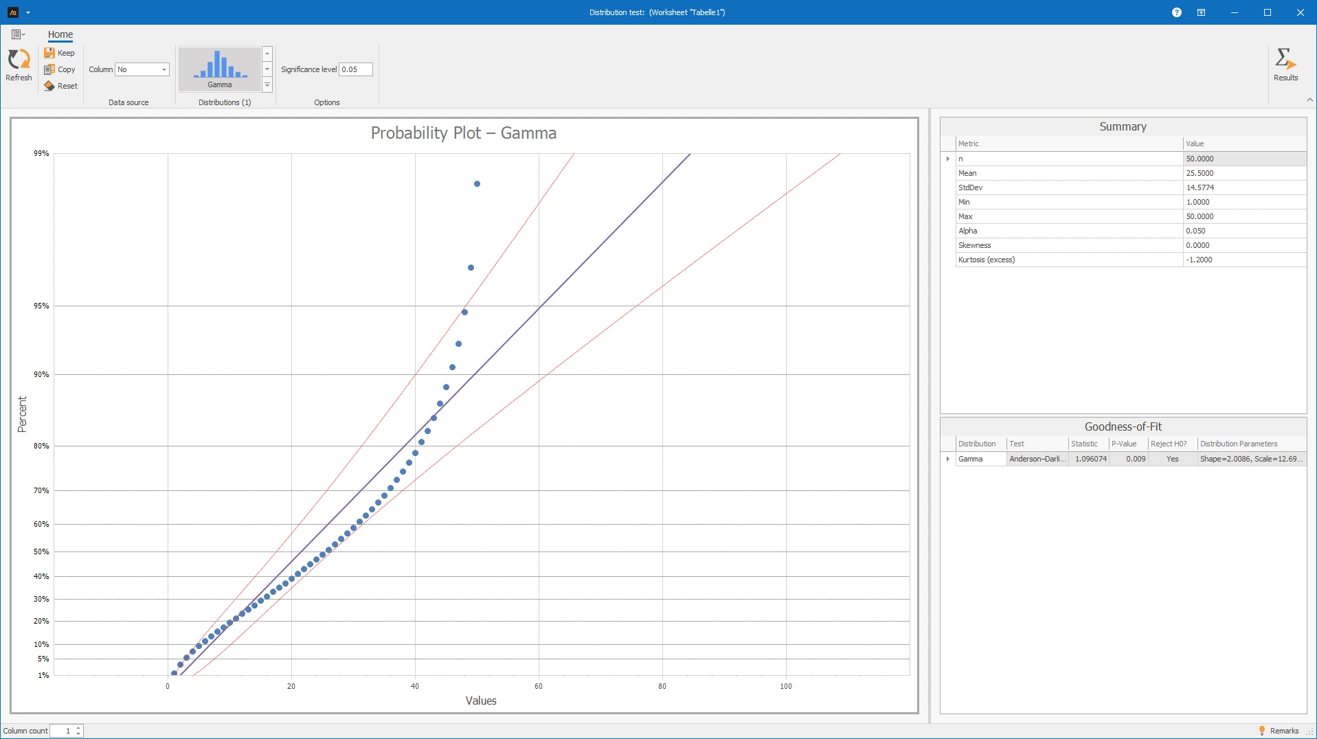
The gamma distribution is used for positive, right-skewed data. It is suitable for measurements such as waiting times, throughput times, quantities, or loads, provided no negative values can occur.
It is more flexible than the exponential distribution because it can take different forms. This allows it to describe both highly skewed and moderately skewed data well.
Lognormal Distribution
The lognormal distribution arises when the logarithmic values are approximately normally distributed. It is used for positive data that are right-skewed.
Typical examples are times, lifetimes, concentrations, costs, or other quantities where very large individual values can occur. If data is not normally distributed, a lognormal distribution may often fit better.
Logistic Distribution
The logistic distribution is symmetric and resembles the normal distribution. However, it has slightly stronger tails, allowing extreme values to occur somewhat more frequently than in the normal distribution.
It can be used when data is generally symmetrically distributed, but the normal distribution does not describe the tails well enough.
Gumbel Distribution
The Gumbel distribution describes maximum values. It is used when particularly high values are the focus, such as maximum loads, peak temperatures, maximum waiting times, or peak values.
It is suitable when not the typical average value, but the behavior of the largest observations is important.
Minimum Extreme Value Distribution
The minimum extreme value distribution describes minimum values. It is used when particularly small values are the focus, such as minimum strengths, lowest lifetimes, or earliest failures.
It is helpful when the risk from very small measurements needs to be assessed, for example, in safety limits or minimum requirements.
For nominal or ordinal data, the distribution test is not meaningful, as these data types cannot be described by continuous distributions such as normal, Weibull, or gamma.
For pure count data or discrete events, it should be checked whether a specific method for discrete distributions is more suitable. The distribution test is designed for the continuous distributions supported in the tool.
The distribution test is more suitable when several possible distributions are to be compared with each other.
Filling quantity tomato sauce
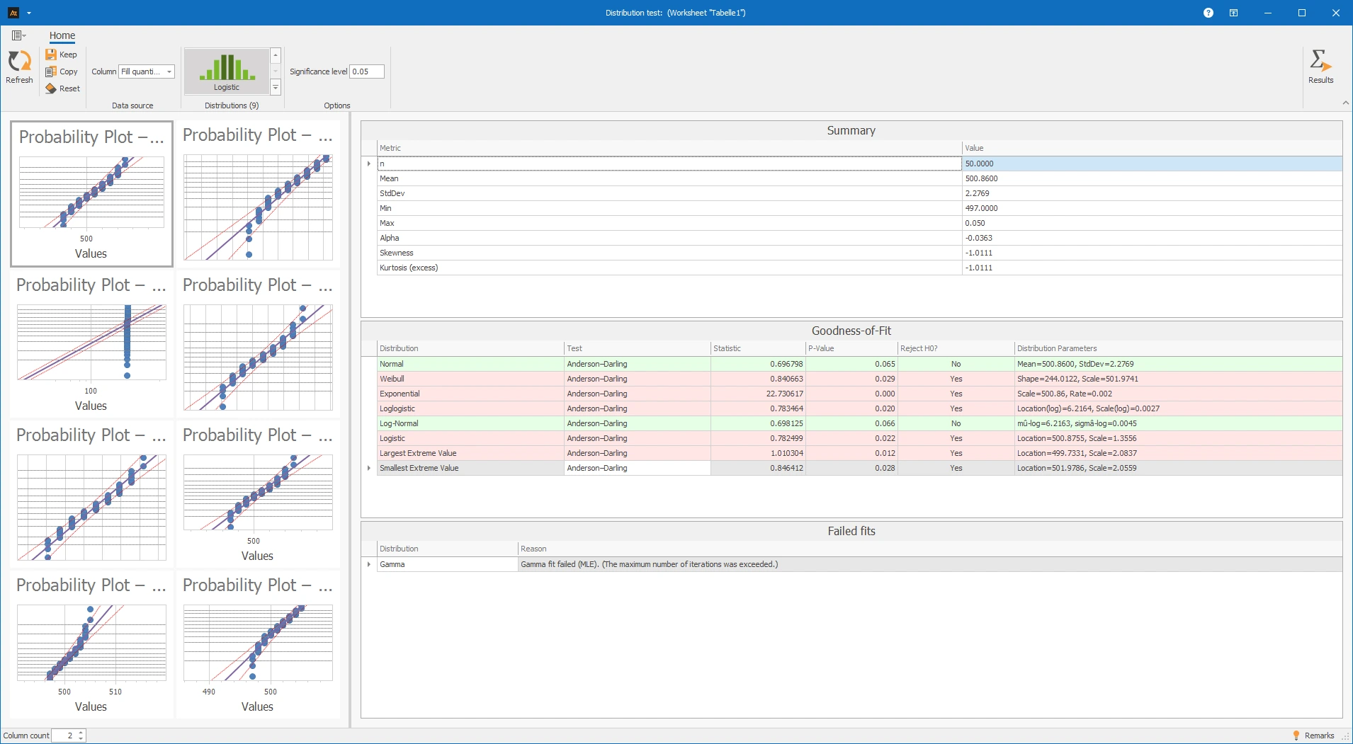
In this example, the filling quantity of a tomato sauce is examined. Each filling should contain 500 ml. Due to normal process fluctuations, some filling quantities are slightly below and others slightly above the target value. Since such measurements often scatter approximately symmetrically around the target value, it is checked which distribution sensibly describes the data. For this purpose, the filling quantities are compared with several distributions, including the normal distribution.
Interpretation
The filling quantities were compared with several distributions. As a result, the normal distribution is not rejected because the p-value of 0.065 is greater than the significance level of 0.05. Also, in the probability plot, the points mostly lie close to the line. Therefore, the filling quantities can be approximately described by a normal distribution.
Several other distributions, on the other hand, are rejected because their p-values are less than or equal to 0.05. These include, among others, Weibull, Exponential, Log-logistic, Logistic, and the largest extreme value distribution. There is statistical evidence for these distributions that they do not adequately describe the data.
The log-normal distribution is also not rejected. However, in terms of filling quantities, the normal distribution is often sensible because it is a continuous measurement that typically scatters around a target value.
The gamma distribution could not be calculated because the fit failed. Therefore, it is not used for interpretation.
Conclusion:
For further analysis, the normal distribution can be used because it is not statistically rejected and fits well with filling quantities.
Lead Time of an Order in Goods Receipt
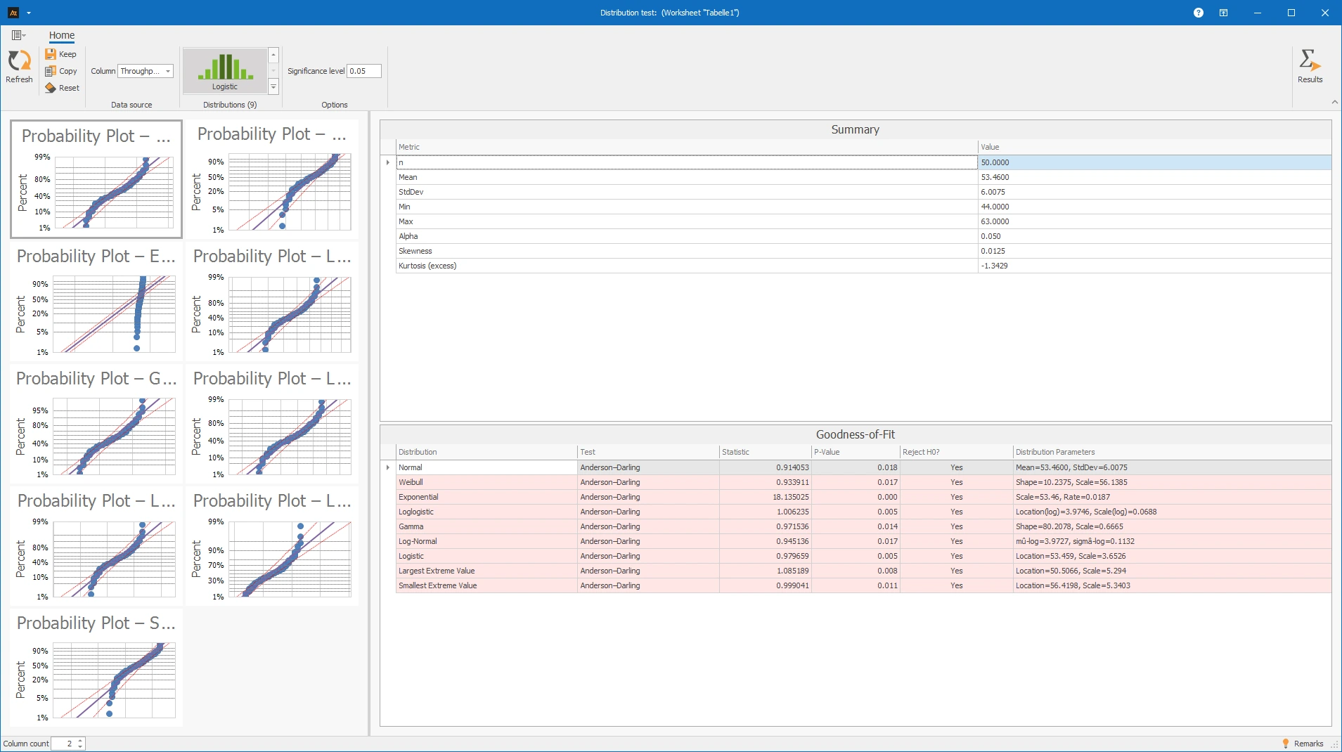
In goods receipt, processing times often have a right-skewed distribution: Many orders are completed quickly, but some processes take significantly longer. Therefore, a log-normal, gamma, Weibull, or exponential distribution may be more plausible than a normal distribution.
Interpretation
The lead times were compared with several distributions. For all tested distributions, the p-value is less than 0.05. Therefore, all distributions are rejected.
Also, in the probability plots, the points do not lie sufficiently well on the lines. Therefore, the data cannot be adequately described by any of the tested distributions.
Conclusion:
None of the tested distributions should be used for the lead times. It should be checked whether different process states or order types cause the variation.
Response time of the IT helpdesk (Specification: max. 35 minutes (OSG))
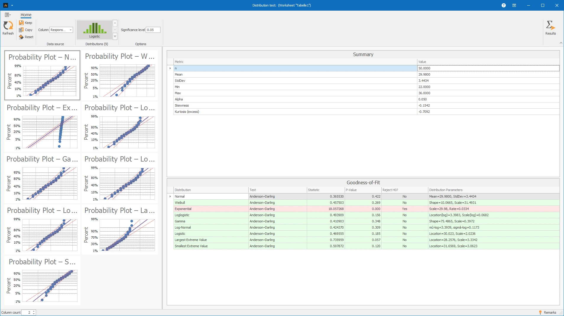
Simple and complex inquiries are received at the IT service desk. This can result in response times that vary around a typical value but also have long right tails. Best Fit helps to check which distribution best describes this behavior.
Interpretation
The response times were compared with several distributions. Most of the tested distributions are not rejected because their p-values are greater than 0.05. Only the exponential distribution is rejected because the p-value is less than 0.05.
For this distribution, the data do not fit sufficiently well. The probability plots also show predominantly points close to the line for the non-rejected distributions.
Conclusion:
The response times can be approximately described by several distributions. For further analysis, a distribution that is appropriate for the subject should be chosen; the exponential distribution should not be used.
Service life of ball bearings
For a new type of machine, ball bearings are tested in continuous operation. Each bearing remains in the test stand until it is no longer functional. Such service life data is typically positive and often not normally distributed.
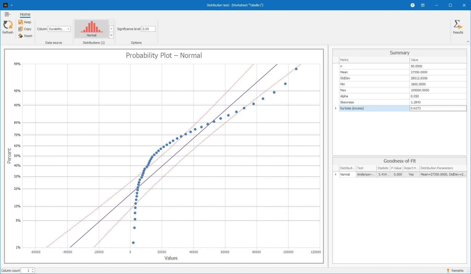
In the probability plot of the normal distribution, the points can deviate significantly from the line. This argues against a normal distribution of the service lives.
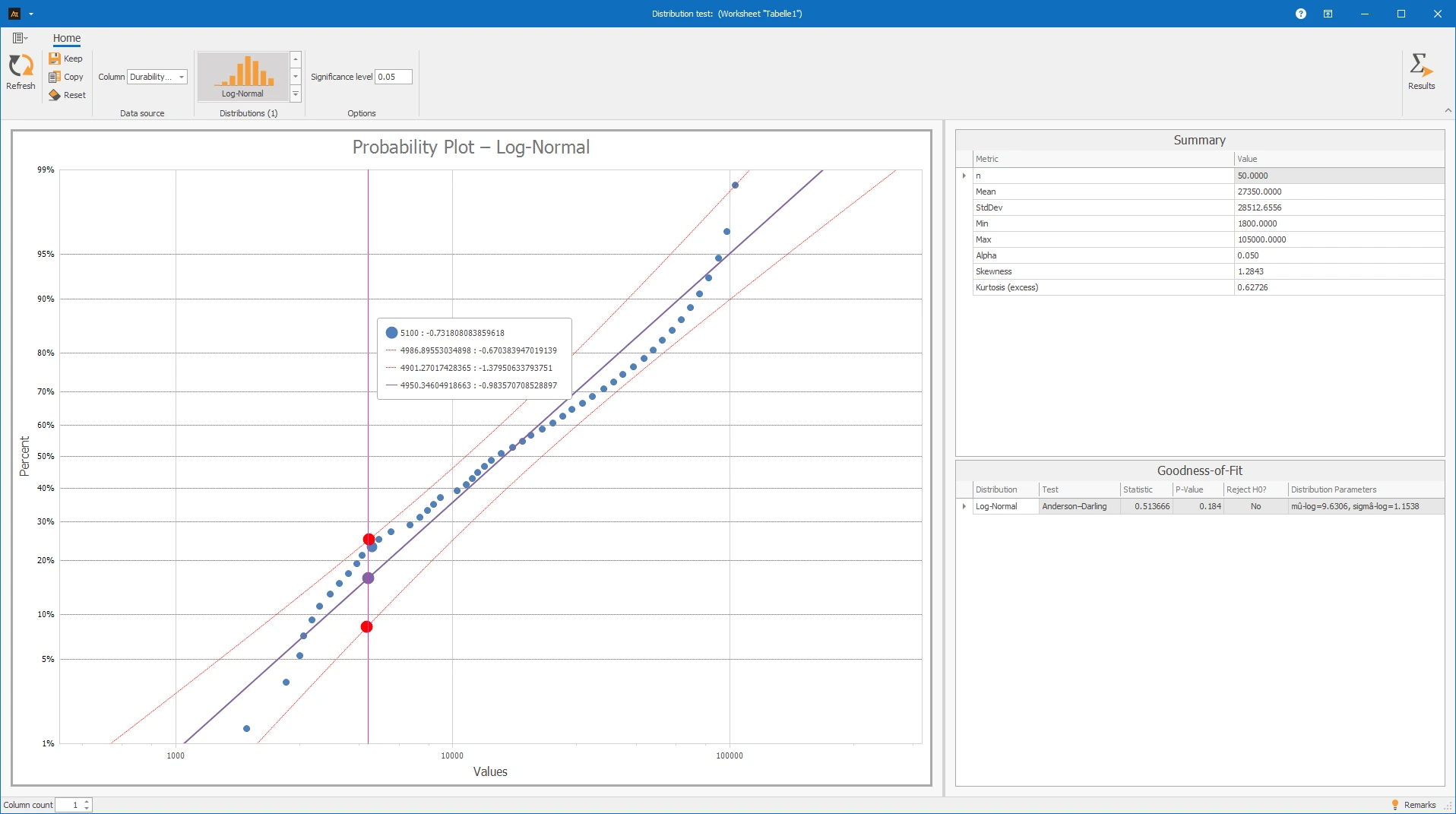
The service life of the ball bearings was tested with the lognormal distribution. The p-value is 0.190 and is therefore greater than 0.05. The lognormal distribution is therefore not rejected.
Also in the probability plot, the points are mostly close to the line. The service life data can therefore be approximately described by a lognormal distribution.
Continuous data: Data collected with a measuring instrument that can have units and decimal places.
Distribution: Mathematical model that describes how measurements typically spread.
Anderson-Darling test: Statistical test to check if data fits a selected distribution.
p-value: Metric for evaluating the test result. The smaller the p-value, the stronger the data speaks against the tested distribution.
A² statistic: Measure of the deviation of the data from the tested distribution. Smaller values tend to indicate less deviation from the tested distribution.
H0: Null hypothesis of the test. It states: The data follows the tested distribution.
n = Sample size: Number of valid measurements in the sample.
Mean: Average of all measurements. It describes the central location of the data.
Standard deviation: Measure of how much the measurements spread around the mean. A small standard deviation means little spread, a large standard deviation means greater spread.
Minimum: Smallest measurement within the considered sample.
Maximum: Largest measurement within the considered sample.
Alpha (α): Set significance level and decision threshold for the p-value. Often α = 0.05 is used. If the p-value is smaller than Alpha, the null hypothesis H0 is rejected.
Skewness: Metric for the symmetry of a distribution. A value near 0 indicates an approximately symmetric distribution. Positive or negative values indicate a stronger expression of the distribution to the right or left, respectively.
Kurtosis: Metric that describes the shape of a distribution, particularly how strongly measurements concentrate in the center and in the tails. It can provide clues as to whether a distribution is more peaked or flat compared to a normal distribution.
The distribution test calculates the corresponding parameters, the test statistic, and the p-value for the selected distributions. Functions from the Numerics.NET library are used to calculate the test statistic.