


The tool is used to plan a study in advance. It calculates the required sample size so that a statistical test can detect a relevant difference, a change in variance, or a change in proportion with sufficient probability.
Unlike power calculation, the focus is not on how powerful a test is with existing data. Instead, it asks how much data is needed to achieve a desired power:
- high desired power → more data is needed
- lower desired power → less data is needed, but the β error is larger
Important: When calculating the sample size, assumptions summarized in AlphadiTab are entered. Therefore, no raw data is needed, but key figures such as expected effect, standard deviation, desired power, significance level, or expected proportions.
In product development, a new tomato sauce formulation is being tested. The goal is to determine whether the viscosity of the new formulation differs on average from the previous formulation.
For this purpose, viscosity measurements are to be carried out on samples of the old formulation and the new formulation.
Before the investigation, it should be planned how many samples per formulation are required to reliably detect a practically relevant difference.
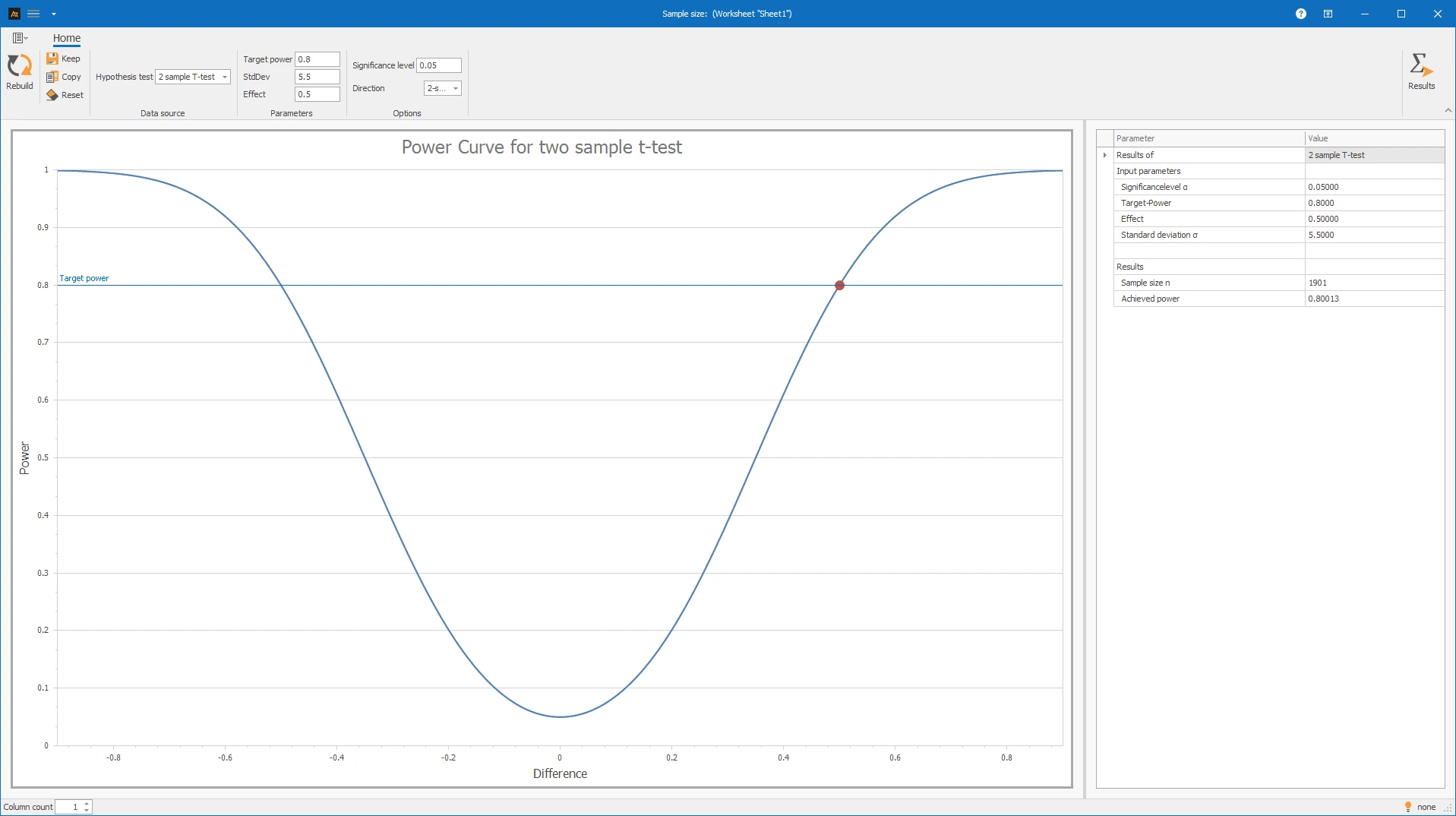
For planning, it must be determined which difference in mean viscosity should be detected. The decisive factor is which difference is practically relevant. In this example, a difference in means of 0.5 MPa is to be detected. This difference corresponds to the effect.
In addition, an expected standard deviation is required. This can be derived, for example, from preliminary tests, previous analyses, or empirical values. In this example, a standard deviation of 5.5 MPa is assumed.
A target power of 80% is set. This means that a truly existing difference of 0.5 MPa should be detected with 80% probability. The corresponding β-error is 20%.
Interpretation of the results:
The result shows that a sample size of 1901 per group is required to detect the assumed difference of 0.5 MPa with the desired power.
If the calculated sample size is very high, it means that the assumed effect is small relative to the variability. In this case, many samples are needed to reliably demonstrate the difference.
Explanations of the graphic:
- The curve shows how the achievable power changes depending on the effect.
- The point marks the calculated case for the chosen inputs.
- The larger the effect, the higher the power is usually with the same sample size.
- For very small effects, larger sample sizes are needed to achieve the desired power.
The following are the considerations and steps necessary to calculate the required sample size for various statistical tests.
Preparation
- Select the appropriate test, e.g., t-test, F-test, test of proportions, or ANOVA.
- Determine which difference, variance ratio, or change in proportions is practically relevant.
- Set the significance level, usually α = 0.05.
- Set the target power, often 80% or 90%.
- Prepare necessary assumptions, e.g., standard deviation, expected proportions, or number of groups.
- Determine the direction of the question, two-sided, greater, or less, if the procedure supports this choice.
 Use in AlphadiTab
- In the Analyze Phase, select the Sample Size tool.
- Select the appropriate test type, e.g., t-test, F-test, test of proportions, or ANOVA.
- Enter the target power, e.g., 0.80 or 0.90.
- Enter the significance level, e.g., 0.05.
- Enter the other summarized metrics into the input fields.
- Conduct the analysis by “Create New”.
Interpretation
- Check what sample size is required.
- Check if the calculated sample size is practically feasible.
- If a very large sample size is required, check if the assumed effect is very small or if the variance can be reduced.
Important: The sample size is a planning parameter. It does not indicate whether an effect actually exists. It describes how much data is needed to detect an assumed effect with the desired power.
Test types
- t-Test: Sample sizes for comparing means.
- F-Test: Sample sizes for comparing variances or dispersions.
- Test of proportions: Sample sizes for comparing ratios or binary events.
- ANOVA: Sample sizes for comparing means from two or more groups.
- Test on variances: Sample sizes for comparing variances or dispersions for two or more samples, optionally also non-parametric.
In hypothesis tests with two samples, the direction for the alternative hypothesis can be selected.
Choose two-sided when a difference is to be detected without specifying a particular direction.
- This setting is useful when both higher and lower values would be relevant.
Example:
Is the average delivery time different between two processes?
Choose greater when an effect is only relevant in the direction of higher values.
- This setting is useful, for example, when testing if a success rate increases.
Example:
Is the sales rate higher with a new sales approach than before?
Choose smaller when an effect is only relevant in the direction of lower values.
- This setting is useful, for example, when testing if a processing time or defect rate decreases.
Example:
Is the average processing time lower after an optimization than before?
Filling quantity tomato sauce – Machine A vs. Machine B
In production, several filling machines are used. It should be planned how many measurements per machine are required to reliably detect a difference between Machine A and Machine B.
t-Test:
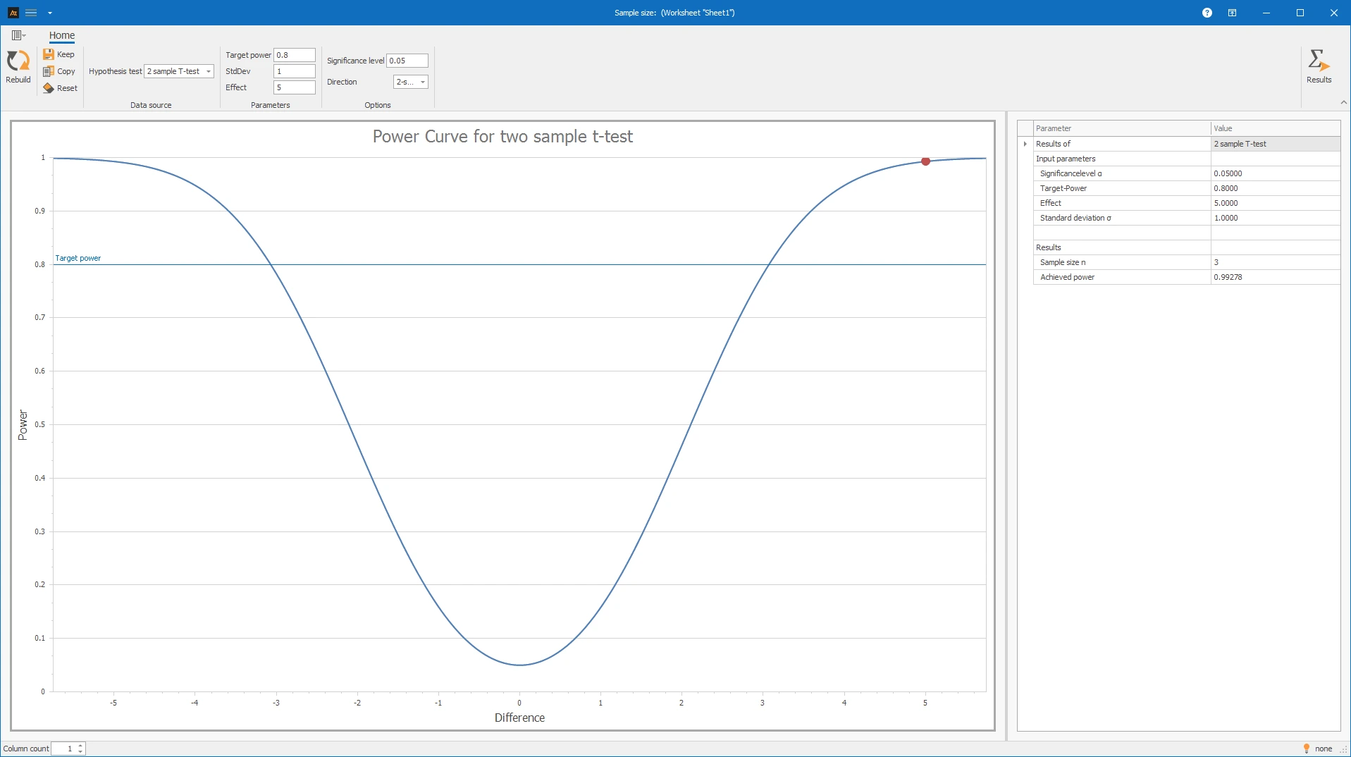
Differences in means: How many measurements per machine are needed to detect a difference of 5 ml in the average filling quantity with 80% power, assuming a standard deviation of 1.1 ml?
Interpretation
For the t-test, the sample size calculation shows how many measurements per machine are required to detect the assumed difference in the average filling quantity. In this case, 3 measurements per machine are needed.
Levene's Test:
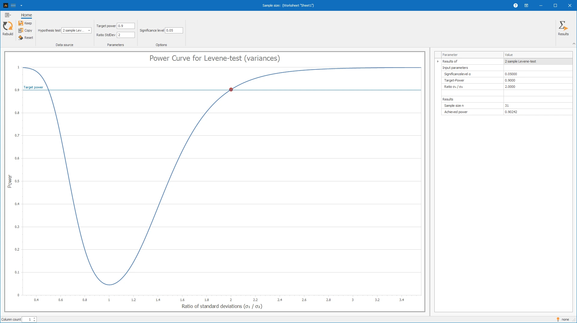
Differences in variances: How many measurements per machine are needed to detect a doubling of the variance of the filling quantity with 90% power?
Interpretation
For Levene's test, the sample size calculation shows how many measurements per group are required to detect a difference in variance. In this example, a doubling of the standard deviation with 90% power is to be detected. The β-error is thus 10%. For this, 31 measurements per machine are needed.
Response time of the IT helpdesk vs. location ANOVA
In the IT service desk, tickets are processed at multiple locations. Response times are regularly evaluated to identify differences in service quality.
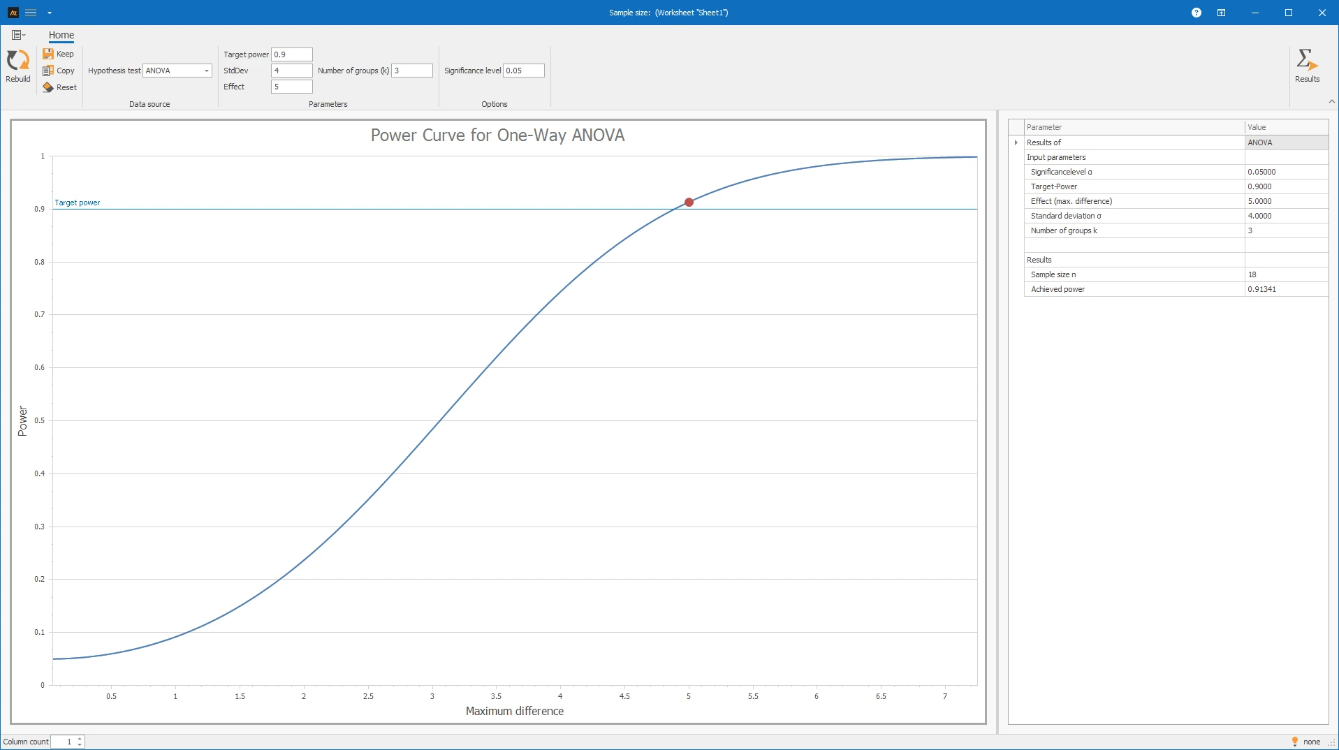
In the example of IT tickets, there are three locations. Using sample size calculation, it is planned how many tickets per location need to be evaluated to detect a difference of 5 minutes in response time with ANOVA. The standard deviation is estimated at 4 minutes and the target power is 90%.
Interpretation of the results
The result shows that 18 tickets per location are required to detect a maximum difference of 5 minutes between the locations with the desired power.
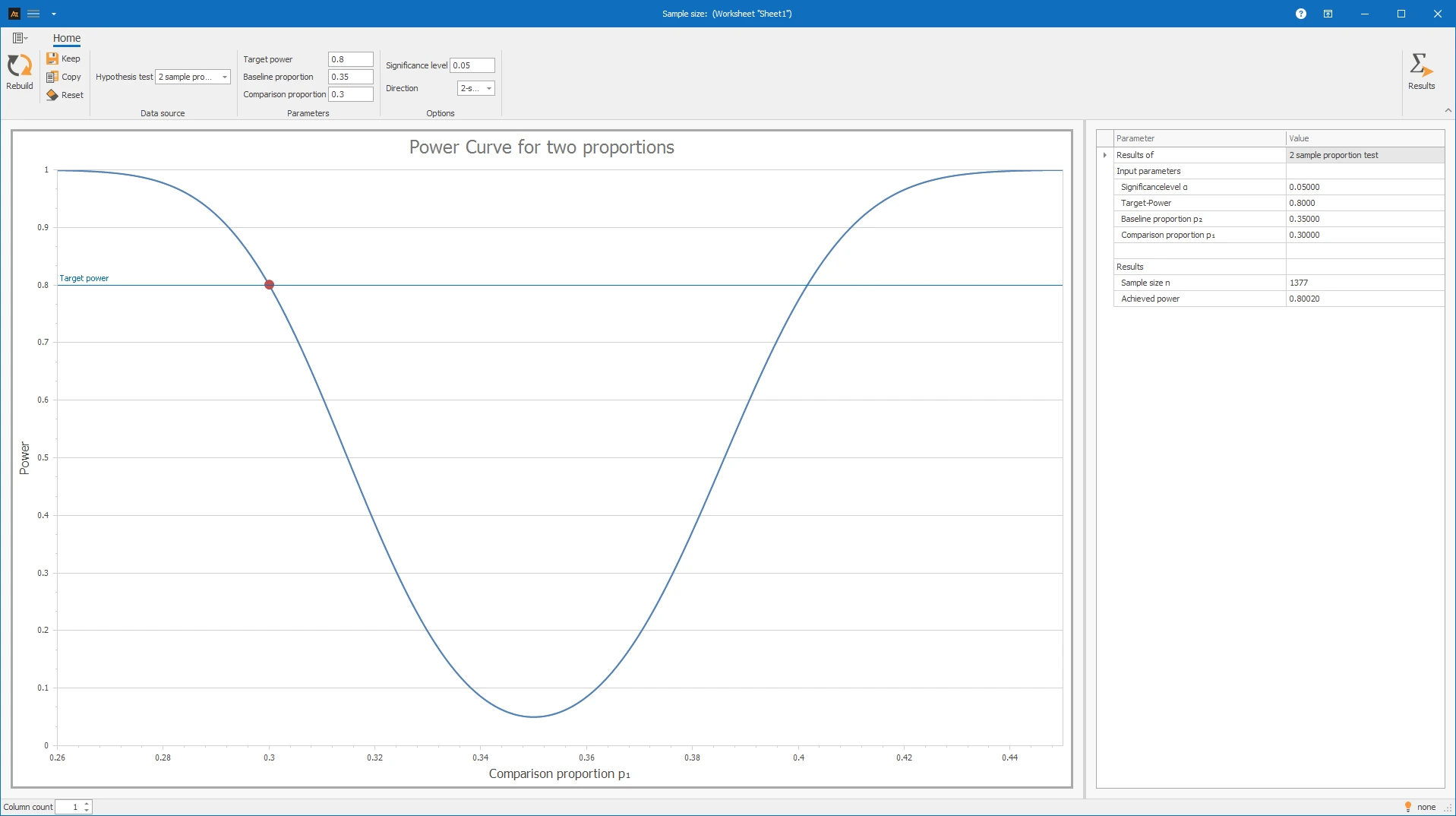
Test of Proportions - Loss Rate by Sales Approach
In sales, two sales approaches are compared. It is planned to determine how many offers need to be evaluated per sales approach to reliably detect a relevant change in the loss rate.
The test of proportions is intended to check whether the loss rate differs between the sales types.
Now, using the sample size calculation, it should be determined how many offers are required to detect a change from 35% to 30% with 80% power.
Interpretation
The sample size calculation indicates how many offers per group are needed for the test to detect a relevant change in the loss rate. In this case, 1377 offers are needed per sales approach.
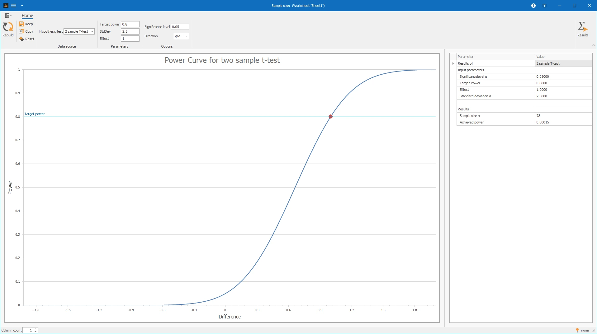
Delivery time after logistics center
In the logistics department, customer orders are picked and shipped. New forklifts have been introduced to increase efficiency.
It is planned to determine how many measurements are needed to detect an improvement in delivery time by 1 day using a one-sided t-test. The variation in delivery time is estimated at 2.5 days.
A target power of 80% is used.
Interpretation
The result shows that 78 measurements are required to detect an improvement in delivery time by 1 day with 80% power.
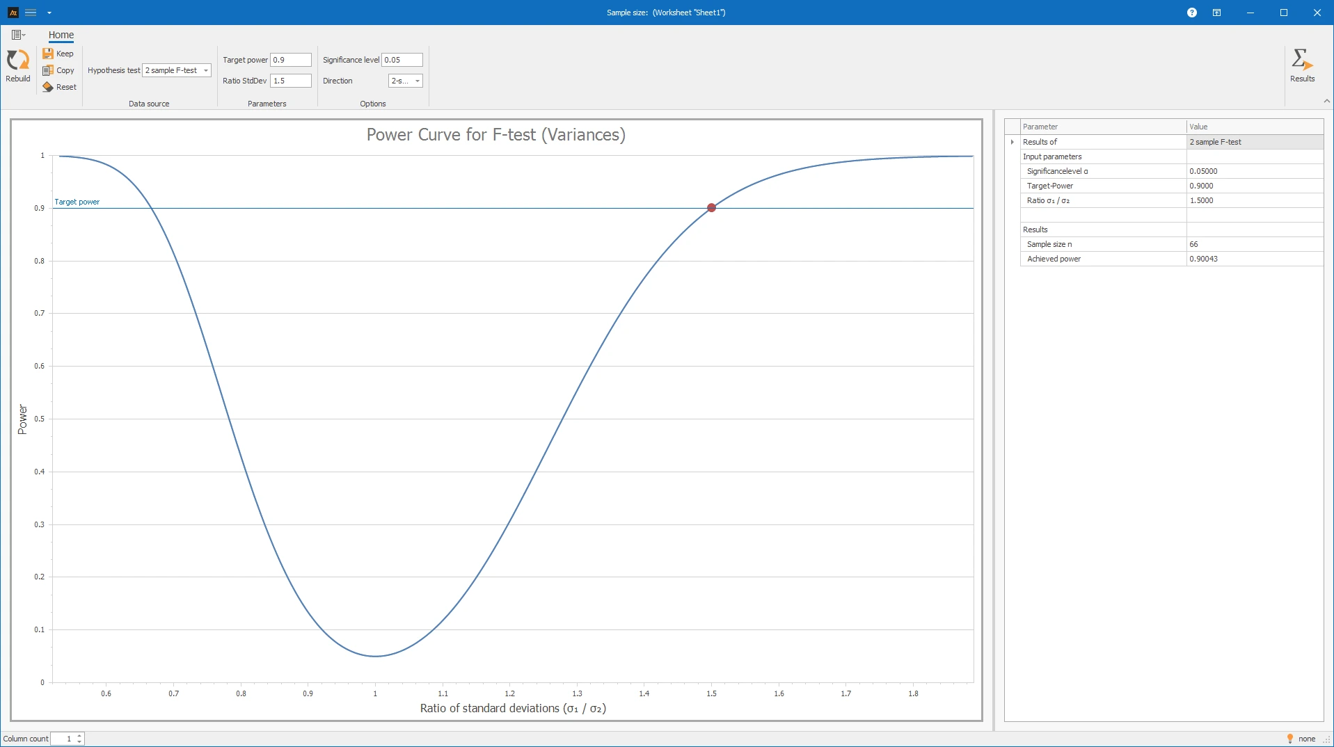
Supplier Comparison
In purchasing, components are sourced from multiple suppliers. It should be planned how many data sets per supplier are required to detect a 1.5-fold difference in the standard deviation between suppliers. The desired discrimination power is 80%.
Interpretation
For a two-sided F-test, 66 data sets are needed to detect a 1.5-fold change in the standard deviation.
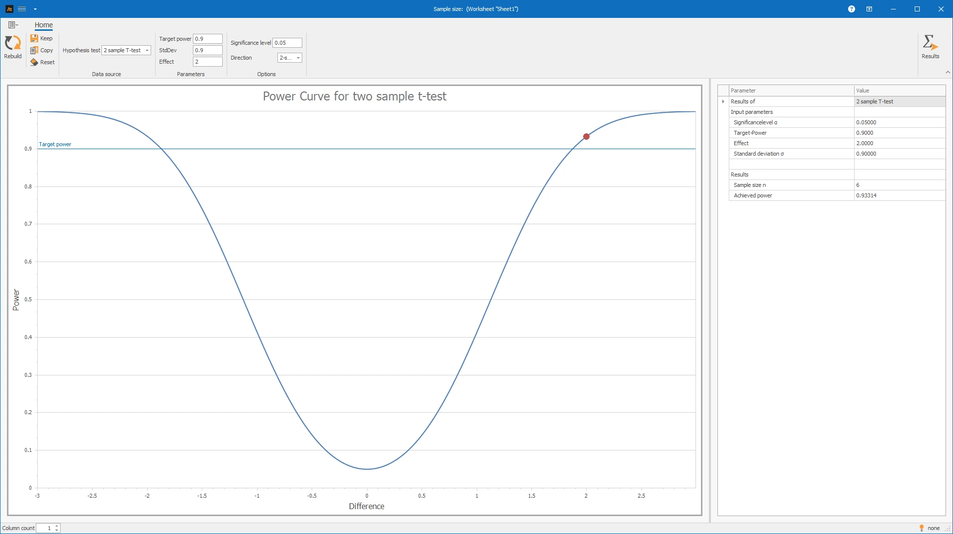
Forecast deviation
In production planning, demand forecasts are created for different planning periods. To assess the quality of the forecast, the forecast deviation is calculated.
It is planned to determine how many forecasts per planning horizon are required to detect differences between short-term and long-term planning horizons with a t-test. A difference of 2% should be detected. The standard deviation is known from previous analyses and is 0.9%.
A target power of 90% is used.
Interpretation
For the planned study, 6 forecasts per planning horizon are needed to detect a difference of 2% with a power of 90%.
A target power of 90% means that the assumed difference will be detected with 90% probability. The β-error is accordingly 10%.
Since the calculated sample size with 6 forecasts per planning horizon is comparatively small, the study can usually be well planned. If the required sample size is significantly higher under other assumptions, it can be checked whether a larger relevant effect can be assumed, the variance can be reduced, or a target power of 80% is sufficient for the question.
Sample Size: Number of observations, parts, offers, measurements, or trials needed to detect an assumed effect with a desired power.
Power: Probability that a test will detect an actually existing effect.
Target Power: Pre-determined power to be achieved with the planned sample, e.g., 80% or 90%.
Effect: Practically relevant difference, e.g., mean difference, variance ratio, or odds change.
α = Significance Level: Pre-specified probability of error with which the null hypothesis is incorrectly rejected.
β = Type II Error: Probability of not detecting an actually existing effect.
Power = 1 - β: Complementary probability to the Type II error.
x̄ = Sample Mean: Average value of the collected measurement data.
s = Sample Standard Deviation: Measure of the dispersion of the data around the mean.
p̂ = Sample Proportion: Proportion of events in a sample; calculated as events / number of trials.
Event: The case of interest in a proportion analysis, e.g., leaking, lost, on time, or passed.
Factor: Categorical influencing variable in ANOVA, e.g., logistics center, supplier, or formulation.
Groups / Levels: Manifestations of the factor, e.g., Center A, Center B, and Center C.
Two-sided: It is tested whether a difference can be detected in both directions.
Greater: It is tested whether an effect can be detected in the direction of greater values.
Smaller: It is tested whether an effect can be detected in the direction of smaller values.
For the sample size calculation, the same calculation formulas are used as for the discrimination power. The required sample size is iteratively adjusted until the specified target discrimination power is achieved.
See the description under Discrimination Power.