Test for variances

Purpose of the tool

The test for variances is used to check whether the dispersions of two or more groups differ statistically significantly. It does not answer the question of whether means differ, but whether the variances or standard deviations are comparable.

The tool is particularly helpful when assessing whether multiple processes, formulations, machines, or groups operate similarly stably or whether one group varies significantly more than the others.

The decision is made by comparing the p-value with the set significance level (usually α = 0.05):

p > α → Retain H₀; there is no significant indication of different variances.
p ≤ α → Reject H₀; there is a significant difference in the variances.

Example viscosity of tomato sauce - multiple formulations

You can download the data here: ViscosityRecipeABC.xlsx

In product development, multiple formulations for tomato sauce are tested. For the same viscosity data, it is now not checked whether the means differ, but whether the dispersion of viscosity between the formulations is of different magnitude.

For this purpose, viscosity measurements are carried out on samples of formulation A, formulation B, and formulation C. The measurements of the groups are collected independently and considered as samples.

Using the test for variances, it should be checked whether the formulations have comparable process dispersion or whether at least one formulation is significantly more variable.

Interpretation of the results:

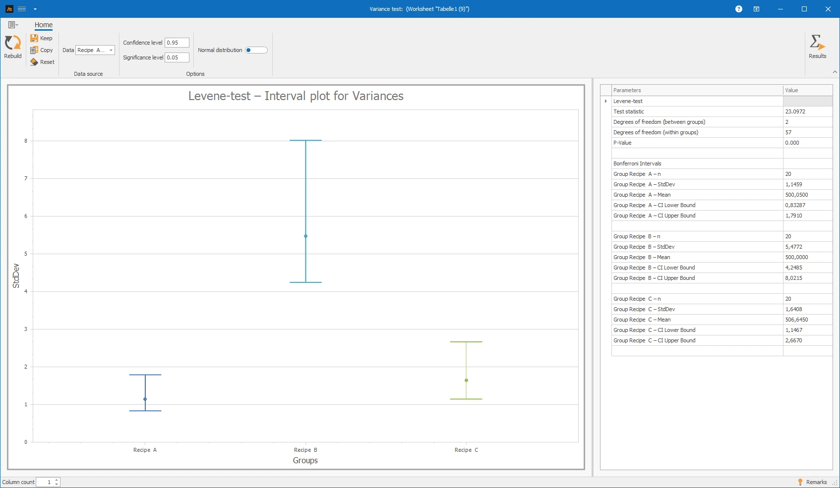
The p-value is compared with the significance level of 0.05. Since the p-value in this example is displayed as 0.000, it is below 0.05. The null hypothesis of equal variances is therefore rejected.

This means: The formulations may not only differ in their average viscosity but also in the dispersion of viscosity values. At least one formulation shows a significantly different dispersion than the remaining formulations.

For product development, this is important because a formulation with high dispersion is less stable. Even if the mean value is generally in the desired range, individual batches can turn out significantly thinner or thicker. A formulation with lower dispersion, on the other hand, is more manageable and delivers more consistent product properties.

The error bar chart shows the standard deviations of the formulations with the associated Bonferroni confidence intervals. Formulations with larger standard deviations exhibit greater fluctuations in viscosity. However, the final statistical decision is made based on the p-value.

Explanations of the graphic:

The points mark the standard deviations of viscosity for the individual formulations.
The error bars represent confidence intervals of the standard deviations. When normal distribution is activated, Bonferroni intervals are used; without activated normal distribution, Bonett intervals are used.
Overlaps of the intervals provide an initial visual indication. The final decision is made based on the p-value.

Procedure

The following are the considerations and steps necessary to conduct a test for variances for two or more samples.

Preparation

Select a continuous measurement variable (e.g., viscosity).
Define two or more groups whose variances are to be compared (e.g., formulation A, B, and C).
Set the significance level (usually α = 0.05).
Set the confidence level (usually 95%).
Check whether the measurements were taken independently of each other.
Decide whether to assume a normal distribution. Without activated normal distribution, the tool uses the Levene test; with activated normal distribution, the F-test is used for two groups and the Bartlett test for more than two groups.

Usage in AlphadiTab

In the Analyze Phase, select the Test for Variances tool.
Under Data, select all groups to be compared.
Set the confidence level and the significance level.
Optionally activate normal distribution if the assumption of normal distribution is justified technically.
Conduct the analysis by “Create New”.

Interpretation

Check which test was applied: Levene test, F-test, or Bartlett test.
Check whether the p-value is less than or equal to the significance level.
p ≤ α → statistically significant difference between at least two variances or standard deviations.
p > α → no statistically significant difference between the variances or standard deviations.

Important: The test for variances first checks the dispersions. It does not make any statement about whether the means of the groups are different.

Requirements

Two or more groups

There must be at least two groups whose variances are to be compared (e.g., formulation A, formulation B, and formulation C).

Why is this important? The test for variances is a procedure for comparing variances between groups. For exactly two groups, an F-test can be used if the normal distribution assumption is met. For multiple groups, the Bartlett test is used for normally distributed data.

Independent samples

The measurements of the groups must not influence each other. There should be no pairings of the same parts or individuals.

Why is this important? The test assumes that the groups were collected independently. Dependent measurements require different procedures.

Continuous measurement data

The measurements must be continuous.

Why is this important? Variance tests compare the spread of numerical measurement data. For pure counts, categories, or proportions, other procedures are more suitable.

Normally distributed data

If the normal distribution option is enabled, the data per group should be approximately normally distributed.

Why is this important? The F-test and the Bartlett test are sensitive to deviations from normal distribution. For skewed distributions, outliers, or uncertain normal distribution assumptions, the Levene test should be preferred. The tool uses the Levene test based on absolute deviations from the median without the normal distribution enabled. This variant is more robust against outliers and non-normality.

When are other tools more suitable?

When the same parts or people are measured multiple times

Procedure for connected measurements

When averages, not variations, are to be compared

ANOVA

t-Test (2 groups)

When proportions or frequencies, not continuous measurements, are to be compared

Two-Proportion Test or Chi-square test

Example in production

Filling quantity tomato sauce – Machine A, Machine B, and Machine C

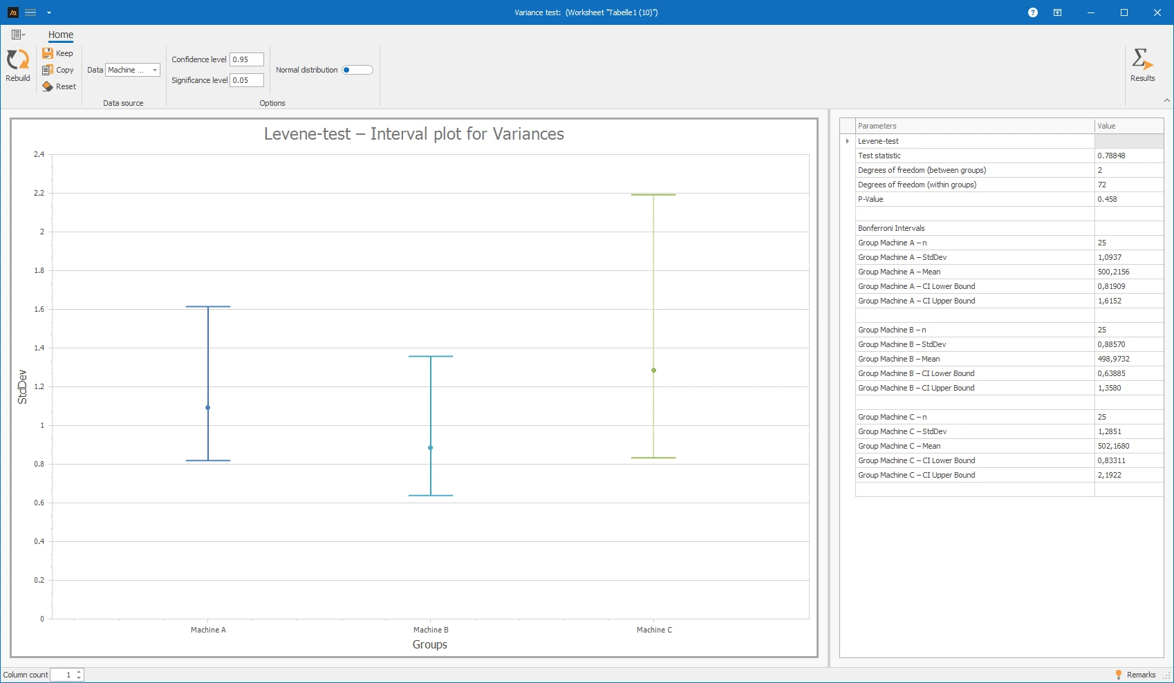
In production, three filling machines are used. It should be investigated whether the filling quantities of the machines vary significantly. While an ANOVA compares the average filling quantities, the test for variances examines the dispersion of the machines.

You can download the data here: FillingQuantityMachineABC.xlsx

Interpretation

The p-value is above 0.05. Therefore, the null hypothesis of equal variances is not rejected.

The filling quantities of the machines do not vary statistically significantly. The machines operate comparably stable in terms of their fluctuation. Differences in the means would need to be tested separately.

Example in IT helpdesks

Response time of the IT helpdesk vs. location

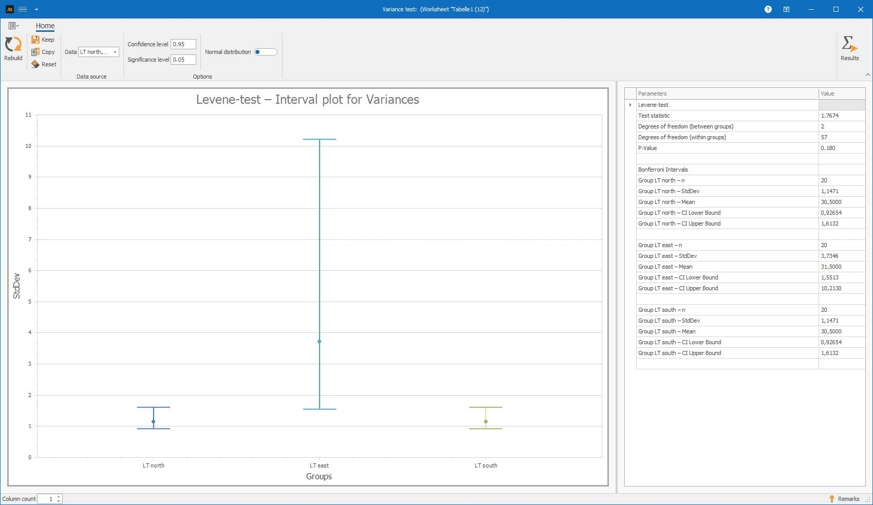
In the IT service desk, tickets are processed at multiple locations. It should be checked whether the response times vary significantly between locations. High variability can indicate inconsistent service processes or highly fluctuating workloads.

You can download the data here: ResponseTimeTicketsLocation.xlsx

Interpretation

The p-value is above 0.05. The null hypothesis of equal variances is not rejected.

The response times of the locations do not vary statistically significantly. A wide confidence interval in the diagram rather indicates an uncertain estimate, for example due to a small sample size or individual outliers. A definite difference in variances cannot be derived from this.

Example in Sales

Lead Time by Region

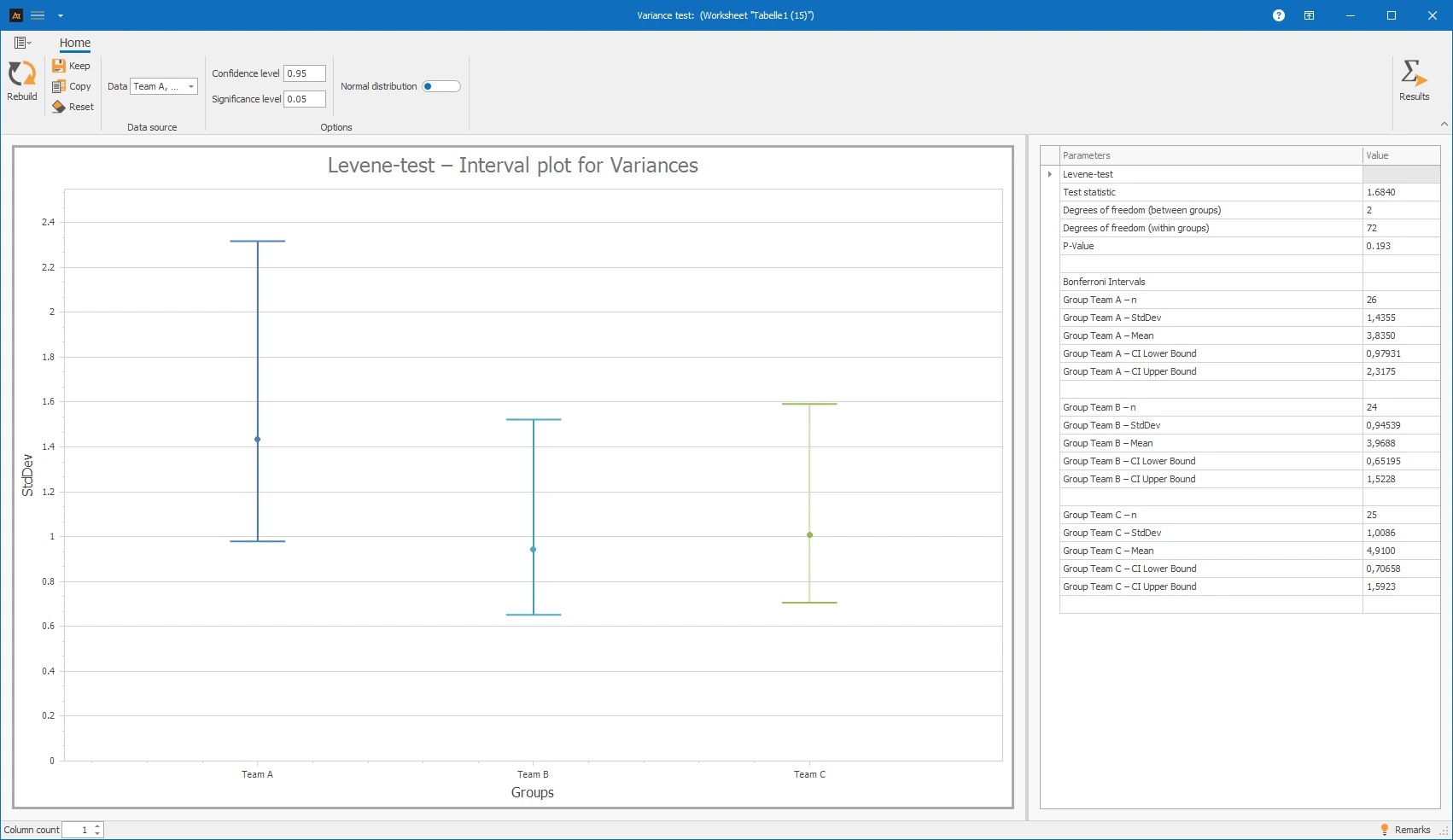
In sales, customer offers are processed by multiple teams. Besides the average lead time, it is also interesting to see whether the processing time is consistent or highly variable.

You can download the data here: VertriebTeams.xlsx

Interpretation

The p-value is above 0.05. The null hypothesis of equal variances is not rejected.

The lead times of the teams do not differ statistically significantly. Thus, there is no indication that one team works significantly more inconsistently or less predictably than the others.

Example in logistics

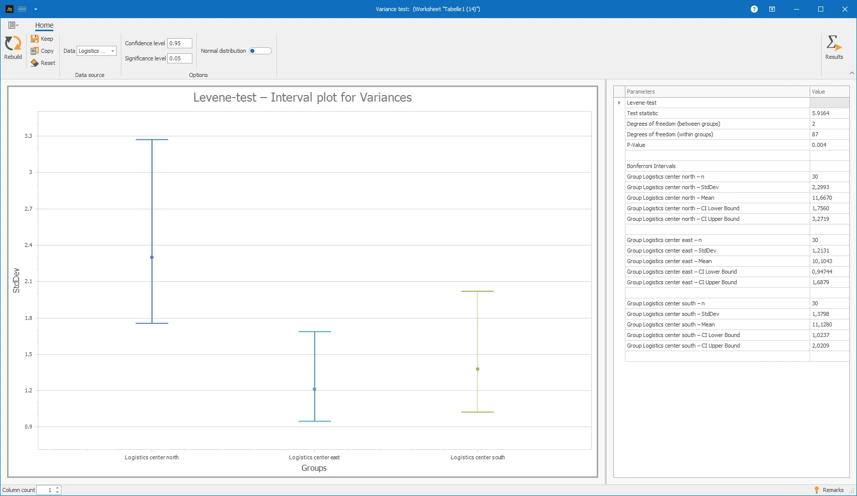
Delivery time after logistics center

In the logistics department, customer orders are picked and shipped. It should be investigated whether the delivery times in the logistics centers vary significantly.

H₀: σ²_Center A = σ²_Center B = σ²_Center C
H₁: At least one variance differs.

You can download the data here: DeliveryTimeLogisticsCenter.xlsx

Interpretation

The p-value is below 0.05. The null hypothesis of equal variances is rejected.

The delivery times vary statistically significantly between the logistics centers. At least one center delivers less consistently. This may indicate differences in workload, processes, or transport conditions.

Example in Purchasing

Supplier Comparison

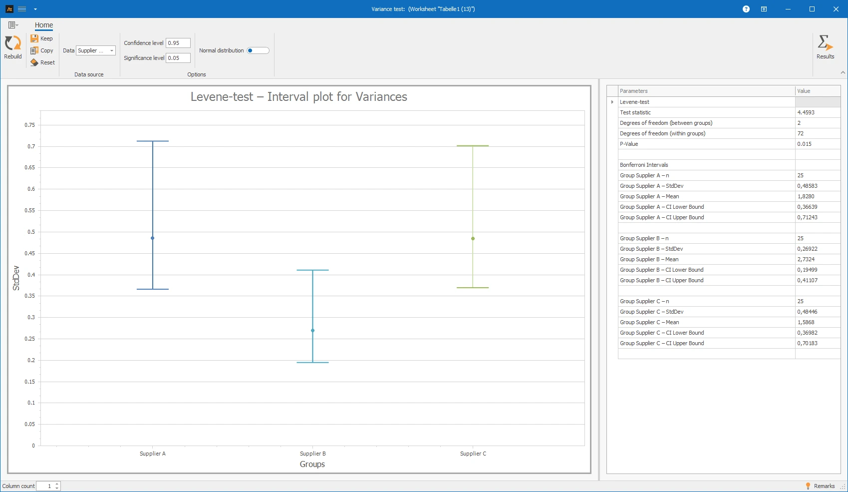
In purchasing, components are sourced from three suppliers. It should be investigated whether the rejection rates per delivery fluctuate more with individual suppliers than with others.

Note:

Percentage values like the rejection rate can be discrete, as they arise from count values. With small delivery quantities, only a few possible percentage values arise. In such cases, the suitability of the test should be professionally examined.

You can download the data here: RejectionSupplierABC.xlsx

Interpretation

The p-value is below 0.05. The null hypothesis of equal variances is rejected.

The rejection rates vary statistically significantly between suppliers. A supplier may be acceptable on average but deliver less reliably because the quality fluctuates more.

Example in planning

Forecast deviation

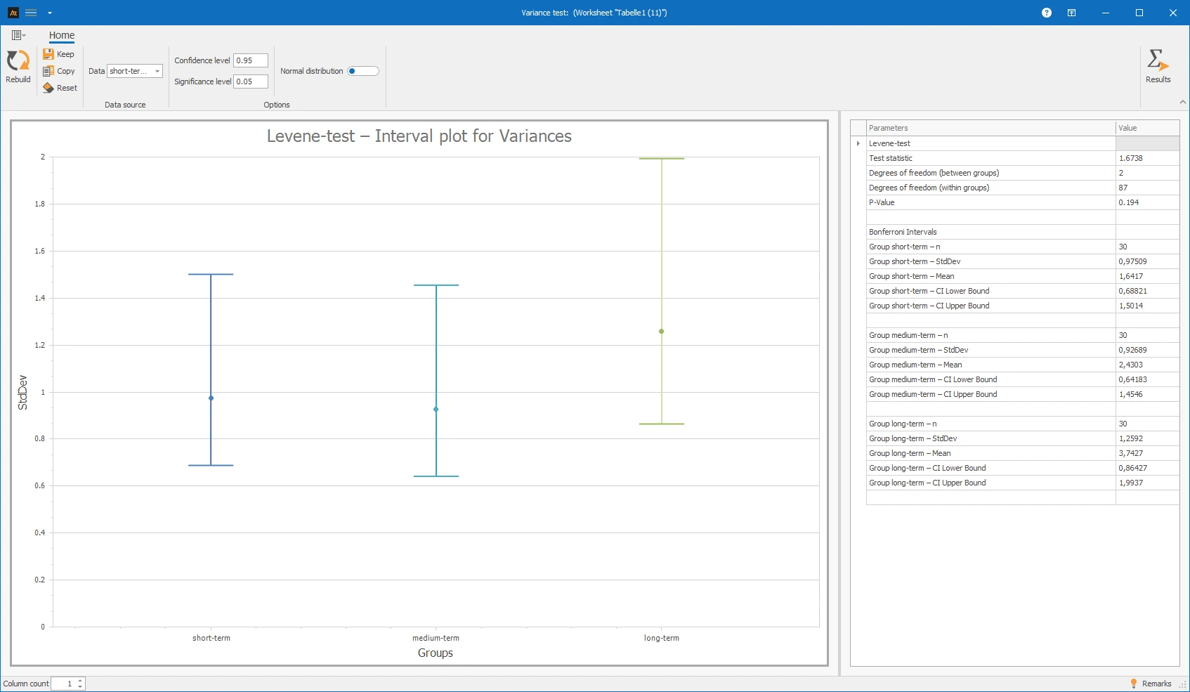
In production planning, demand forecasts are created for different planning periods. It should be investigated whether the forecast deviations vary significantly between short-term, medium-term, and long-term planning horizons.

You can download the data here: PlanningHorizonDeviation.xlsx

Interpretation

The p-value of 0.194 is above the significance level of 0.05. Therefore, the null hypothesis of equal variances is not rejected.

Thus, there is no statistically significant evidence that the spread of forecast deviations differs between planning horizons. Differences in the range of variation may be visible in the sample, but they are not statistically confirmed based on this test.

Terms

Continuous data: Data collected with a measuring instrument that can have both units and decimal places.

Normally distributed data: Data that can be well described by a normal distribution. This can be checked, for example, through a test for normal distribution or through suitable diagrams.

s: Standard deviation of the sample. It describes the dispersion of the measurements around the mean.

s²: Variance of the sample. It is the square of the standard deviation.

n: Sample size. Number of observations within a sample.

α: Significance level. Preset probability of error with which the null hypothesis is incorrectly rejected.

p-value: Result of the hypothesis test used to make a decision between the null hypothesis and the alternative hypothesis.

F-value: Test statistic in the F-test or Levene's test. In the F-test, it describes the ratio of two sample variances.

Chi-square value: Test statistic in the Bartlett test for more than two groups under the assumption of normal distribution.

df: Degrees of freedom. Values derived from the number of groups and observations that determine the shape of the test distribution.

Confidence level: Probability with which the calculated confidence interval covers the true parameter value (e.g., 95%).

Confidence interval: Range of values that contains the true standard deviation or variance with the chosen confidence level.

Null hypothesis: Initial hypothesis that assumes equal variances for all groups when testing variances.

Alternative hypothesis: Counter-hypothesis to the null hypothesis. It states that at least one variance differs from the others.

Levene's test: Robust test for equality of variances. In the tool, the absolute deviations from the group median are used.

F-test: Test for equality of two variances under the assumption of normal distribution.

Bartlett test: Test for equality of multiple variances under the assumption of normal distribution.

Bonferroni intervals: Adjusted confidence intervals that take into account the overall error probability when comparing multiple groups simultaneously.

Formulas

The test for equality of variances checks whether the variances of several groups differ statistically significantly.

With the normal distribution assumption enabled, the tool uses the F-test for exactly two groups and the Bartlett test for more than two groups. Without the normal distribution assumption enabled, a median-based Levene test is used.

The required distribution and quantile functions of the F, Chi-square, and normal distribution are evaluated using CenterSpace NMath.

Hypotheses

H₀: σ₁² = σ₂² = … = σ_k²

H₁: At least one variance σ_i² differs.

Notation

σ_i² = Variance of group i

k = Number of groups

F-test for two normally distributed groups

If exactly two groups are present and the Normal distribution option is enabled, the tool uses a two-sided F-test.

F = s₁² / s₂²

Notation

s₁² = Sample variance of the first group

s₂² = Sample variance of the second group

df₁ = n₁ − 1

df₂ = n₂ − 1

The p-value is determined two-sided from the F-distribution. The distribution function of the F-distribution is evaluated using CenterSpace NMath.

F ≥ 1: p = 2 · [1 − F_df1,df2(F)]

F < 1: p = 2 · F_df1,df2(F)

Notation

F_df1,df2(x) = Distribution function of the F-distribution

Bartlett test for multiple normally distributed groups

If more than two groups are present and the Normal distribution option is enabled, the tool uses the Bartlett test.

First, the pooled variance is calculated:

s_p² = [Σ_i=1^k (n_i − 1) s_i²] / [Σ_i=1^k (n_i − 1)]

The Bartlett test statistic used in the tool is:

B = { [Σ(n_i − 1)] · ln(s_p²) − Σ(n_i − 1) ln(s_i²) } / C

C = 1 + [1 / (3(k − 1))] · { Σ[1/(n_i − 1)] − 1 / Σ(n_i − 1) }

Notation

s_i² = Variance of group i

s_p² = Pooled variance

n_i = Sample size of group i

k = Number of groups

Under the null hypothesis, the test statistic is approximately evaluated with a Chi-square distribution with k − 1 degrees of freedom. The Chi-square distribution function is calculated using CenterSpace NMath.

p = 1 − F_χ²,k−1(B)

Levene test without normal distribution assumption

If the Normal distribution option is not enabled, the tool uses a median-based variant of the Levene test. First, the absolute deviations from the respective group median are calculated for each group.

z_ij = |x_ij − Median_i|

Notation

x_ij = Observation j in group i

Median_i = Median of group i

z_ij = Absolute deviation from the group median

A one-way ANOVA is then applied to the absolute deviations. The test statistic is derived from the ratio of the mean squares between and within the groups.

F = MS_between / MS_within

df_between = k − 1
df_within = N − k

Notation

k = Number of groups

N = Total number of observations

The p-value is determined from the right tail of the F-distribution. The F-distribution function is evaluated using CenterSpace NMath.

p = 1 − F_k−1,N−k(F)

Bonferroni confidence intervals

In addition to the variance test, the tool calculates a simultaneous confidence interval of the standard deviation for each group. The global error level is distributed among the groups according to Bonferroni.

α_Group = (1 − Confidence level) / k

Notation

k = Number of groups

α_Group = Bonferroni-corrected error level per group

Intervals with normal distribution assumption

With the normal distribution assumption enabled, Chi-square-based confidence intervals for the variance are calculated. The required quantiles of the Chi-square distribution are determined using CenterSpace NMath.

Var_lower = [(n − 1)s²] / χ²_{1−αGroup/2, n−1}

Var_upper = [(n − 1)s²] / χ²_{αGroup/2, n−1}

The limits for the standard deviation are obtained by taking the square root:

SD_lower = √(Var_lower)

SD_upper = √(Var_upper)

Bonett intervals without normal distribution assumption

Without the normal distribution assumption enabled, the tool uses Bonett intervals. Sample size and kurtosis of the respective group are considered.

For larger samples, a trimmed mean is first determined. For samples with at most five observations, the ordinary mean is used.

p = 1 / [2√(n − 4)]

Notation

p = Proportion of observations to be trimmed at both ends

An excess kurtosis is determined from the deviations from the trimmed mean:

γ_e = [n / (n − 1)²] · Σ [((x_i − x̄_trim) / s)&sup4;] − 3

The standard error is then calculated:

SE = √[ (γ_e + 2 + 3/n) / (n − 1) ]

The required quantile of the standard normal distribution is determined using CenterSpace NMath:

z = z_{1−αGroup/2}

The Bonett correction factor used in the tool is:

c = n / (n − z)

The variance limits are then calculated as:

Var_lower = c · s² · exp(−c · z · SE)

Var_upper = c · s² · exp(c · z · SE)

The limits for the standard deviation are again obtained from the square roots of the variance limits.

SD_lower = √(Var_lower)

SD_upper = √(Var_upper)